
Big Data Analytics - Summarizing Data
Reporting is very important in big data analytics. Every organization must have a regular provision of information to support its decision making process. This task is normally handled by data analysts with SQL and ETL (extract, transfer, and load) experience.
The team in charge of this task has the responsibility of spreading the information produced in the big data analytics department to different areas of the organization.
The following example demonstrates what summarization of data means. Navigate to the folder bda/part1/summarize_data and inside the folder, open the summarize_data.Rproj file by double clicking it. Then, open the summarize_data.R script and take a look at the code, and follow the explanations presented.
# Install the following packages by running the following code in R.
pkgs = c('data.table', 'ggplot2', 'nycflights13', 'reshape2')
install.packages(pkgs)
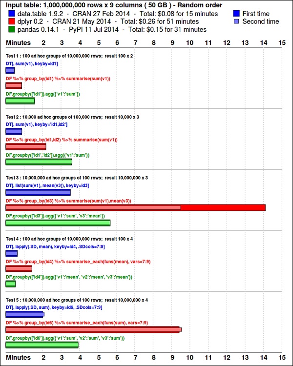
The ggplot2 package is great for data visualization. The data.table package is a great option to do fast and memory efficient summarization in R. A recent benchmark shows it is even faster than pandas, the python library used for similar tasks.
Take a look at the data using the following code. This code is also available in bda/part1/summarize_data/summarize_data.Rproj file.
library(nycflights13)
library(ggplot2)
library(data.table)
library(reshape2)

# Convert the flights data.frame to a data.table object and call it DT
DT <- as.data.table(flights)

# The data has 336776 rows and 16 columns
dim(DT)

# Take a look at the first rows
head(DT)

#   year    month  day   dep_time  dep_delay  arr_time  arr_delay  carrier
# 1: 2013     1     1      517       2         830         11       UA
# 2: 2013     1     1      533       4         850         20       UA
# 3: 2013     1     1      542       2         923         33       AA
# 4: 2013     1     1      544      -1        1004        -18       B6
# 5: 2013     1     1      554      -6         812        -25       DL
# 6: 2013     1     1      554      -4         740         12       UA

#     tailnum  flight  origin   dest    air_time   distance    hour   minute
# 1:  N14228   1545     EWR      IAH      227        1400       5       17
# 2:  N24211   1714     LGA      IAH      227        1416       5       33
# 3:  N619AA   1141     JFK      MIA      160        1089       5       42
# 4:  N804JB    725     JFK      BQN      183        1576       5       44
# 5:  N668DN    461     LGA      ATL      116        762        5       54
# 6:  N39463   1696     EWR      ORD      150        719        5       54
The following code has an example of data summarization.
### Data Summarization
# Compute the mean arrival delay
DT[, list(mean_arrival_delay = mean(arr_delay, na.rm = TRUE))]
#        mean_arrival_delay
# 1:           6.895377
# Now, we compute the same value but for each carrier
mean1 = DT[, list(mean_arrival_delay = mean(arr_delay, na.rm = TRUE)),
   by = carrier]
print(mean1)
#      carrier    mean_arrival_delay
# 1:      UA          3.5580111
# 2:      AA          0.3642909
# 3:      B6          9.4579733
# 4:      DL          1.6443409
# 5:      EV         15.7964311
# 6:      MQ         10.7747334
# 7:      US          2.1295951
# 8:      WN          9.6491199
# 9:      VX          1.7644644
# 10:     FL         20.1159055
# 11:     AS         -9.9308886
# 12:     9E          7.3796692
# 13:     F9         21.9207048
# 14:     HA         -6.9152047
# 15:     YV         15.5569853
# 16:     OO         11.9310345

# Now let’s compute to means in the same line of code
mean2 = DT[, list(mean_departure_delay = mean(dep_delay, na.rm = TRUE),
   mean_arrival_delay = mean(arr_delay, na.rm = TRUE)),
   by = carrier]
print(mean2)

#       carrier    mean_departure_delay   mean_arrival_delay
# 1:      UA            12.106073          3.5580111
# 2:      AA             8.586016          0.3642909
# 3:      B6            13.022522          9.4579733
# 4:      DL             9.264505          1.6443409
# 5:      EV            19.955390         15.7964311
# 6:      MQ            10.552041         10.7747334
# 7:      US             3.782418          2.1295951
# 8:      WN            17.711744          9.6491199
# 9:      VX            12.869421          1.7644644
# 10:     FL            18.726075         20.1159055
# 11:     AS             5.804775         -9.9308886
# 12:     9E            16.725769          7.3796692
# 13:     F9            20.215543         21.9207048
# 14:     HA             4.900585         -6.9152047
# 15:     YV            18.996330         15.5569853
# 16:     OO            12.586207         11.9310345

### Create a new variable called gain
# this is the difference between arrival delay and departure delay
DT[, gain:= arr_delay - dep_delay]

# Compute the median gain per carrier
median_gain = DT[, median(gain, na.rm = TRUE), by = carrier]
print(median_gain)


