
Big Data Analytics - Time Series Analysis
Time series is a sequence of observations of categorical or numeric variables indexed by a date, or timestamp. A clear example of time series data is the time series of a stock price. In the following table, we can see the basic structure of time series data. In this case the observations are recorded every hour.
| Timestamp | Stock - Price |
|---|---|
| 2015-10-11 09:00:00 | 100 |
| 2015-10-11 10:00:00 | 110 |
| 2015-10-11 11:00:00 | 105 |
| 2015-10-11 12:00:00 | 90 |
| 2015-10-11 13:00:00 | 120 |
Normally, the first step in time series analysis is to plot the series, this is normally done with a line chart.
The most common application of time series analysis is forecasting future values of a numeric value using the temporal structure of the data. This means, the available observations are used to predict values from the future.
The temporal ordering of the data, implies that traditional regression methods are not useful. In order to build robust forecast, we need models that take into account the temporal ordering of the data.
The most widely used model for Time Series Analysis is called Autoregressive Moving Average (ARMA). The model consists of two parts, an autoregressive (AR) part and a moving average (MA) part. The model is usually then referred to as the ARMA(p, q) model where p is the order of the autoregressive part and q is the order of the moving average part.
Autoregressive Model
The AR(p) is read as an autoregressive model of order p. Mathematically it is written as −
$$X_t = c + \sum_{i = 1}^{P} \phi_i X_{t - i} + \varepsilon_{t}$$
where {φ1, …, φp} are parameters to be estimated, c is a constant, and the random variable εt represents the white noise. Some constraints are necessary on the values of the parameters so that the model remains stationary.
Moving Average
The notation MA(q) refers to the moving average model of order q −
$$X_t = \mu + \varepsilon_t + \sum_{i = 1}^{q} \theta_i \varepsilon_{t - i}$$
where the θ1, ..., θq are the parameters of the model, μ is the expectation of Xt, and the εt, εt − 1, ... are, white noise error terms.
Autoregressive Moving Average
The ARMA(p, q) model combines p autoregressive terms and q moving-average terms. Mathematically the model is expressed with the following formula −
$$X_t = c + \varepsilon_t + \sum_{i = 1}^{P} \phi_iX_{t - 1} + \sum_{i = 1}^{q} \theta_i \varepsilon_{t-i}$$
We can see that the ARMA(p, q) model is a combination of AR(p) and MA(q) models.
To give some intuition of the model consider that the AR part of the equation seeks to estimate parameters for Xt − i observations of in order to predict the value of the variable in Xt. It is in the end a weighted average of the past values. The MA section uses the same approach but with the error of previous observations, εt − i. So in the end, the result of the model is a weighted average.
The following code snippet demonstrates how to implement an ARMA(p, q) in R.
# install.packages("forecast")
library("forecast")
# Read the data
data = scan('fancy.dat')
ts_data <- ts(data, frequency = 12, start = c(1987,1))
ts_data
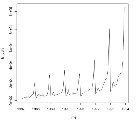
plot.ts(ts_data)
Plotting the data is normally the first step to find out if there is a temporal structure in the data. We can see from the plot that there are strong spikes at the end of each year.
The following code fits an ARMA model to the data. It runs several combinations of models and selects the one that has less error.
# Fit the ARMA model
fit = auto.arima(ts_data)
summary(fit)

# Series: ts_data
# ARIMA(1,1,1)(0,1,1)[12]
#    Coefficients:
#    ar1     ma1    sma1
# 0.2401  -0.9013  0.7499
# s.e.  0.1427   0.0709  0.1790

#
# sigma^2 estimated as 15464184:  log likelihood = -693.69
# AIC = 1395.38   AICc = 1395.98   BIC = 1404.43

# Training set error measures:
#                 ME        RMSE      MAE        MPE        MAPE      MASE       ACF1
# Training set   328.301  3615.374  2171.002  -2.481166  15.97302  0.4905797 -0.02521172


