
Data Structures & Algorithms - Quick Guide
Data Structures & Algorithms - Overview
Data Structure is a systematic way to organize data in order to use it efficiently. Following terms are the foundation terms of a data structure.
Interface − Each data structure has an interface. Interface represents the set of operations that a data structure supports. An interface only provides the list of supported operations, type of parameters they can accept and return type of these operations.
Implementation − Implementation provides the internal representation of a data structure. Implementation also provides the definition of the algorithms used in the operations of the data structure.
Characteristics of a Data Structure
Correctness − Data structure implementation should implement its interface correctly.
Time Complexity − Running time or the execution time of operations of data structure must be as small as possible.
Space Complexity − Memory usage of a data structure operation should be as little as possible.
Need for Data Structure
As applications are getting complex and data rich, there are three common problems that applications face now-a-days.
Data Search − Consider an inventory of 1 million(106) items of a store. If the application is to search an item, it has to search an item in 1 million(106) items every time slowing down the search. As data grows, search will become slower.
Processor speed − Processor speed although being very high, falls limited if the data grows to billion records.
Multiple requests − As thousands of users can search data simultaneously on a web server, even the fast server fails while searching the data.
To solve the above-mentioned problems, data structures come to rescue. Data can be organized in a data structure in such a way that all items may not be required to be searched, and the required data can be searched almost instantly.
Execution Time Cases
There are three cases which are usually used to compare various data structure's execution time in a relative manner.
Worst Case − This is the scenario where a particular data structure operation takes maximum time it can take. If an operation's worst case time is ƒ(n) then this operation will not take more than ƒ(n) time where ƒ(n) represents function of n.
Average Case − This is the scenario depicting the average execution time of an operation of a data structure. If an operation takes ƒ(n) time in execution, then m operations will take mƒ(n) time.
Best Case − This is the scenario depicting the least possible execution time of an operation of a data structure. If an operation takes ƒ(n) time in execution, then the actual operation may take time as the random number which would be maximum as ƒ(n).
Basic Terminology
Data − Data are values or set of values.
Data Item − Data item refers to single unit of values.
Group Items − Data items that are divided into sub items are called as Group Items.
Elementary Items − Data items that cannot be divided are called as Elementary Items.
Attribute and Entity − An entity is that which contains certain attributes or properties, which may be assigned values.
Entity Set − Entities of similar attributes form an entity set.
Field − Field is a single elementary unit of information representing an attribute of an entity.
Record − Record is a collection of field values of a given entity.
File − File is a collection of records of the entities in a given entity set.
Data Structures - Environment Setup
Try it Option Online
You really do not need to set up your own environment to start learning C programming language. Reason is very simple, we already have set up C Programming environment online, so that you can compile and execute all the available examples online at the same time when you are doing your theory work. This gives you confidence in what you are reading and to check the result with different options. Feel free to modify any example and execute it online.
Try the following example using the Try it option available at the top right corner of the sample code box −
#include <stdio.h>
int main(){
   /* My first program in C */
   printf("Hello, World! \n");
   return 0;
}
For most of the examples given in this tutorial, you will find Try it option, so just make use of it and enjoy your learning.
Local Environment Setup
If you are still willing to set up your environment for C programming language, you need the following two tools available on your computer, (a) Text Editor and (b) The C Compiler.
Text Editor
This will be used to type your program. Examples of few editors include Windows Notepad, OS Edit command, Brief, Epsilon, EMACS, and vim or vi.
The name and the version of the text editor can vary on different operating systems. For example, Notepad will be used on Windows, and vim or vi can be used on Windows as well as Linux or UNIX.
The files you create with your editor are called source files and contain program source code. The source files for C programs are typically named with the extension ".c".
Before starting your programming, make sure you have one text editor in place and you have enough experience to write a computer program, save it in a file, compile it, and finally execute it.
The C Compiler
The source code written in the source file is the human readable source for your program. It needs to be "compiled", to turn into machine language so that your CPU can actually execute the program as per the given instructions.
This C programming language compiler will be used to compile your source code into a final executable program. We assume you have the basic knowledge about a programming language compiler.
Most frequently used and free available compiler is GNU C/C++ compiler. Otherwise, you can have compilers either from HP or Solaris if you have respective Operating Systems (OS).
The following section guides you on how to install GNU C/C++ compiler on various OS. We are mentioning C/C++ together because GNU GCC compiler works for both C and C++ programming languages.
Installation on UNIX/Linux
If you are using Linux or UNIX, then check whether GCC is installed on your system by entering the following command from the command line −
$ gcc -v
If you have GNU compiler installed on your machine, then it should print a message such as the following −
Using built-in specs.
Target: i386-redhat-linux
Configured with: ../configure --prefix = /usr .......
Thread model: posix
gcc version 4.1.2 20080704 (Red Hat 4.1.2-46)
If GCC is not installed, then you will have to install it yourself using the detailed instructions available at https://gcc.gnu.org/install/
This tutorial has been written based on Linux and all the given examples have been compiled on Cent OS flavor of Linux system.
Installation on Mac OS
If you use Mac OS X, the easiest way to obtain GCC is to download the Xcode development environment from Apple's website and follow the simple installation instructions. Once you have Xcode setup, you will be able to use GNU compiler for C/C++.
Xcode is currently available at developer.apple.com/technologies/tools/
Installation on Windows
To install GCC on Windows, you need to install MinGW. To install MinGW, go to the MinGW homepage, www.mingw.org, and follow the link to the MinGW download page. Download the latest version of the MinGW installation program, which should be named MinGW-<version>.exe.
While installing MinWG, at a minimum, you must install gcc-core, gcc-g++, binutils, and the MinGW runtime, but you may wish to install more.
Add the bin subdirectory of your MinGW installation to your PATH environment variable, so that you can specify these tools on the command line by their simple names.
When the installation is complete, you will be able to run gcc, g++, ar, ranlib, dlltool, and several other GNU tools from the Windows command line.
Data Structures - Algorithms Basics
Algorithm is a step-by-step procedure, which defines a set of instructions to be executed in a certain order to get the desired output. Algorithms are generally created independent of underlying languages, i.e. an algorithm can be implemented in more than one programming language.
From the data structure point of view, following are some important categories of algorithms −
Search − Algorithm to search an item in a data structure.
Sort − Algorithm to sort items in a certain order.
Insert − Algorithm to insert item in a data structure.
Update − Algorithm to update an existing item in a data structure.
Delete − Algorithm to delete an existing item from a data structure.
Characteristics of an Algorithm
Not all procedures can be called an algorithm. An algorithm should have the following characteristics −
Unambiguous − Algorithm should be clear and unambiguous. Each of its steps (or phases), and their inputs/outputs should be clear and must lead to only one meaning.
Input − An algorithm should have 0 or more well-defined inputs.
Output − An algorithm should have 1 or more well-defined outputs, and should match the desired output.
Finiteness − Algorithms must terminate after a finite number of steps.
Feasibility − Should be feasible with the available resources.
Independent − An algorithm should have step-by-step directions, which should be independent of any programming code.
How to Write an Algorithm?
There are no well-defined standards for writing algorithms. Rather, it is problem and resource dependent. Algorithms are never written to support a particular programming code.
As we know that all programming languages share basic code constructs like loops (do, for, while), flow-control (if-else), etc. These common constructs can be used to write an algorithm.
We write algorithms in a step-by-step manner, but it is not always the case. Algorithm writing is a process and is executed after the problem domain is well-defined. That is, we should know the problem domain, for which we are designing a solution.
Example
Let's try to learn algorithm-writing by using an example.
Problem − Design an algorithm to add two numbers and display the result.
Step 1 − START
Step 2 − declare three integers a, b & c
Step 3 − define values of a & b
Step 4 − add values of a & b
Step 5 − store output of step 4 to c
Step 6 − print c
Step 7 − STOP
Algorithms tell the programmers how to code the program. Alternatively, the algorithm can be written as −
Step 1 − START ADD
Step 2 − get values of a & b
Step 3 − c ← a + b
Step 4 − display c
Step 5 − STOP
In design and analysis of algorithms, usually the second method is used to describe an algorithm. It makes it easy for the analyst to analyze the algorithm ignoring all unwanted definitions. He can observe what operations are being used and how the process is flowing.
Writing step numbers, is optional.
We design an algorithm to get a solution of a given problem. A problem can be solved in more than one ways.
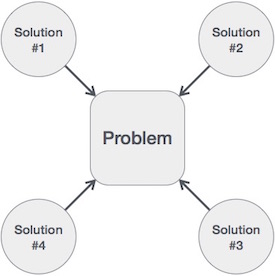
Hence, many solution algorithms can be derived for a given problem. The next step is to analyze those proposed solution algorithms and implement the best suitable solution.
Algorithm Analysis
Efficiency of an algorithm can be analyzed at two different stages, before implementation and after implementation. They are the following −
A Priori Analysis − This is a theoretical analysis of an algorithm. Efficiency of an algorithm is measured by assuming that all other factors, for example, processor speed, are constant and have no effect on the implementation.
A Posterior Analysis − This is an empirical analysis of an algorithm. The selected algorithm is implemented using programming language. This is then executed on target computer machine. In this analysis, actual statistics like running time and space required, are collected.
We shall learn about a priori algorithm analysis. Algorithm analysis deals with the execution or running time of various operations involved. The running time of an operation can be defined as the number of computer instructions executed per operation.
Algorithm Complexity
Suppose X is an algorithm and n is the size of input data, the time and space used by the algorithm X are the two main factors, which decide the efficiency of X.
Time Factor − Time is measured by counting the number of key operations such as comparisons in the sorting algorithm.
Space Factor − Space is measured by counting the maximum memory space required by the algorithm.
The complexity of an algorithm f(n) gives the running time and/or the storage space required by the algorithm in terms of n as the size of input data.
Space Complexity
Space complexity of an algorithm represents the amount of memory space required by the algorithm in its life cycle. The space required by an algorithm is equal to the sum of the following two components −
A fixed part that is a space required to store certain data and variables, that are independent of the size of the problem. For example, simple variables and constants used, program size, etc.
A variable part is a space required by variables, whose size depends on the size of the problem. For example, dynamic memory allocation, recursion stack space, etc.
Space complexity S(P) of any algorithm P is S(P) = C + SP(I), where C is the fixed part and S(I) is the variable part of the algorithm, which depends on instance characteristic I. Following is a simple example that tries to explain the concept −
Algorithm: SUM(A, B)
Step 1 -  START
Step 2 -  C ← A + B + 10
Step 3 -  Stop
Here we have three variables A, B, and C and one constant. Hence S(P) = 1 + 3. Now, space depends on data types of given variables and constant types and it will be multiplied accordingly.
Time Complexity
Time complexity of an algorithm represents the amount of time required by the algorithm to run to completion. Time requirements can be defined as a numerical function T(n), where T(n) can be measured as the number of steps, provided each step consumes constant time.
For example, addition of two n-bit integers takes n steps. Consequently, the total computational time is T(n) = c ∗ n, where c is the time taken for the addition of two bits. Here, we observe that T(n) grows linearly as the input size increases.
Data Structures - Asymptotic Analysis
Asymptotic analysis of an algorithm refers to defining the mathematical boundation/framing of its run-time performance. Using asymptotic analysis, we can very well conclude the best case, average case, and worst case scenario of an algorithm.
Asymptotic analysis is input bound i.e., if there's no input to the algorithm, it is concluded to work in a constant time. Other than the "input" all other factors are considered constant.
Asymptotic analysis refers to computing the running time of any operation in mathematical units of computation. For example, the running time of one operation is computed as f(n) and may be for another operation it is computed as g(n2). This means the first operation running time will increase linearly with the increase in n and the running time of the second operation will increase exponentially when n increases. Similarly, the running time of both operations will be nearly the same if n is significantly small.
Usually, the time required by an algorithm falls under three types −
Best Case − Minimum time required for program execution.
Average Case − Average time required for program execution.
Worst Case − Maximum time required for program execution.
Asymptotic Notations
Following are the commonly used asymptotic notations to calculate the running time complexity of an algorithm.
- Ο Notation
- Ω Notation
- θ Notation
Big Oh Notation, Ο
The notation Ο(n) is the formal way to express the upper bound of an algorithm's running time. It measures the worst case time complexity or the longest amount of time an algorithm can possibly take to complete.
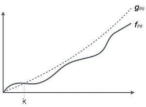
For example, for a function f(n)
Ο(f(n)) = { g(n) : there exists c > 0 and n0 such that f(n) ≤ c.g(n) for all n > n0. }
Omega Notation, Ω
The notation Ω(n) is the formal way to express the lower bound of an algorithm's running time. It measures the best case time complexity or the best amount of time an algorithm can possibly take to complete.
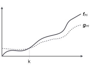
For example, for a function f(n)
Ω(f(n)) ≥ { g(n) : there exists c > 0 and n0 such that g(n) ≤ c.f(n) for all n > n0. }
Theta Notation, θ
The notation θ(n) is the formal way to express both the lower bound and the upper bound of an algorithm's running time. It is represented as follows −
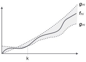
θ(f(n)) = { g(n) if and only if g(n) = Ο(f(n)) and g(n) = Ω(f(n)) for all n > n0. }
Common Asymptotic Notations
Following is a list of some common asymptotic notations −
| constant | − | Ο(1) |
| logarithmic | − | Ο(log n) |
| linear | − | Ο(n) |
| n log n | − | Ο(n log n) |
| quadratic | − | Ο(n2) |
| cubic | − | Ο(n3) |
| polynomial | − | nΟ(1) |
| exponential | − | 2Ο(n) |
Data Structures - Greedy Algorithms
An algorithm is designed to achieve optimum solution for a given problem. In greedy algorithm approach, decisions are made from the given solution domain. As being greedy, the closest solution that seems to provide an optimum solution is chosen.
Greedy algorithms try to find a localized optimum solution, which may eventually lead to globally optimized solutions. However, generally greedy algorithms do not provide globally optimized solutions.
Counting Coins
This problem is to count to a desired value by choosing the least possible coins and the greedy approach forces the algorithm to pick the largest possible coin. If we are provided coins of ₹ 1, 2, 5 and 10 and we are asked to count ₹ 18 then the greedy procedure will be −
1 − Select one ₹ 10 coin, the remaining count is 8
2 − Then select one ₹ 5 coin, the remaining count is 3
3 − Then select one ₹ 2 coin, the remaining count is 1
4 − And finally, the selection of one ₹ 1 coins solves the problem
Though, it seems to be working fine, for this count we need to pick only 4 coins. But if we slightly change the problem then the same approach may not be able to produce the same optimum result.
For the currency system, where we have coins of 1, 7, 10 value, counting coins for value 18 will be absolutely optimum but for count like 15, it may use more coins than necessary. For example, the greedy approach will use 10 + 1 + 1 + 1 + 1 + 1, total 6 coins. Whereas the same problem could be solved by using only 3 coins (7 + 7 + 1)
Hence, we may conclude that the greedy approach picks an immediate optimized solution and may fail where global optimization is a major concern.
Examples
Most networking algorithms use the greedy approach. Here is a list of few of them −
- Travelling Salesman Problem
- Prim's Minimal Spanning Tree Algorithm
- Kruskal's Minimal Spanning Tree Algorithm
- Dijkstra's Minimal Spanning Tree Algorithm
- Graph - Map Coloring
- Graph - Vertex Cover
- Knapsack Problem
- Job Scheduling Problem
There are lots of similar problems that uses the greedy approach to find an optimum solution.
Data Structures - Divide and Conquer
In divide and conquer approach, the problem in hand, is divided into smaller sub-problems and then each problem is solved independently. When we keep on dividing the subproblems into even smaller sub-problems, we may eventually reach a stage where no more division is possible. Those "atomic" smallest possible sub-problem (fractions) are solved. The solution of all sub-problems is finally merged in order to obtain the solution of an original problem.
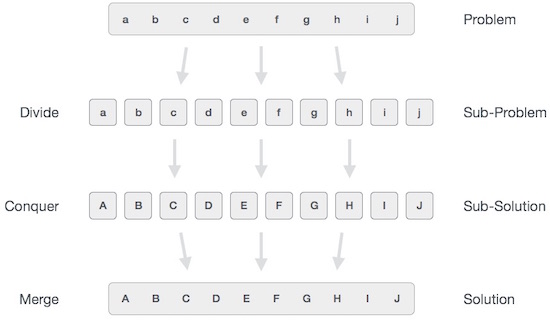
Broadly, we can understand divide-and-conquer approach in a three-step process.
Divide/Break
This step involves breaking the problem into smaller sub-problems. Sub-problems should represent a part of the original problem. This step generally takes a recursive approach to divide the problem until no sub-problem is further divisible. At this stage, sub-problems become atomic in nature but still represent some part of the actual problem.
Conquer/Solve
This step receives a lot of smaller sub-problems to be solved. Generally, at this level, the problems are considered 'solved' on their own.
Merge/Combine
When the smaller sub-problems are solved, this stage recursively combines them until they formulate a solution of the original problem. This algorithmic approach works recursively and conquer & merge steps works so close that they appear as one.
Examples
The following computer algorithms are based on divide-and-conquer programming approach −
- Merge Sort
- Quick Sort
- Binary Search
- Strassen's Matrix Multiplication
- Closest pair (points)
There are various ways available to solve any computer problem, but the mentioned are a good example of divide and conquer approach.
Data Structures - Dynamic Programming
Dynamic programming approach is similar to divide and conquer in breaking down the problem into smaller and yet smaller possible sub-problems. But unlike, divide and conquer, these sub-problems are not solved independently. Rather, results of these smaller sub-problems are remembered and used for similar or overlapping sub-problems.
Dynamic programming is used where we have problems, which can be divided into similar sub-problems, so that their results can be re-used. Mostly, these algorithms are used for optimization. Before solving the in-hand sub-problem, dynamic algorithm will try to examine the results of the previously solved sub-problems. The solutions of sub-problems are combined in order to achieve the best solution.
So we can say that −
The problem should be able to be divided into smaller overlapping sub-problem.
An optimum solution can be achieved by using an optimum solution of smaller sub-problems.
Dynamic algorithms use Memoization.
Comparison
In contrast to greedy algorithms, where local optimization is addressed, dynamic algorithms are motivated for an overall optimization of the problem.
In contrast to divide and conquer algorithms, where solutions are combined to achieve an overall solution, dynamic algorithms use the output of a smaller sub-problem and then try to optimize a bigger sub-problem. Dynamic algorithms use Memoization to remember the output of already solved sub-problems.
Example
The following computer problems can be solved using dynamic programming approach −
- Fibonacci number series
- Knapsack problem
- Tower of Hanoi
- All pair shortest path by Floyd-Warshall
- Shortest path by Dijkstra
- Project scheduling
Dynamic programming can be used in both top-down and bottom-up manner. And of course, most of the times, referring to the previous solution output is cheaper than recomputing in terms of CPU cycles.
Data Structures & Algorithm Basic Concepts
This chapter explains the basic terms related to data structure.
Data Definition
Data Definition defines a particular data with the following characteristics.
Atomic − Definition should define a single concept.
Traceable − Definition should be able to be mapped to some data element.
Accurate − Definition should be unambiguous.
Clear and Concise − Definition should be understandable.
Data Object
Data Object represents an object having a data.
Data Type
Data type is a way to classify various types of data such as integer, string, etc. which determines the values that can be used with the corresponding type of data, the type of operations that can be performed on the corresponding type of data. There are two data types −
- Built-in Data Type
- Derived Data Type
Built-in Data Type
Those data types for which a language has built-in support are known as Built-in Data types. For example, most of the languages provide the following built-in data types.
- Integers
- Boolean (true, false)
- Floating (Decimal numbers)
- Character and Strings
Derived Data Type
Those data types which are implementation independent as they can be implemented in one or the other way are known as derived data types. These data types are normally built by the combination of primary or built-in data types and associated operations on them. For example −
- List
- Array
- Stack
- Queue
Basic Operations
The data in the data structures are processed by certain operations. The particular data structure chosen largely depends on the frequency of the operation that needs to be performed on the data structure.
- Traversing
- Searching
- Insertion
- Deletion
- Sorting
- Merging
Data Structures and Algorithms - Arrays
Array is a container which can hold a fix number of items and these items should be of the same type. Most of the data structures make use of arrays to implement their algorithms. Following are the important terms to understand the concept of Array.
Element − Each item stored in an array is called an element.
Index − Each location of an element in an array has a numerical index, which is used to identify the element.
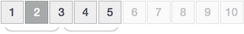
Array Representation
Arrays can be declared in various ways in different languages. For illustration, let's take C array declaration.
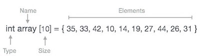
Arrays can be declared in various ways in different languages. For illustration, let's take C array declaration.
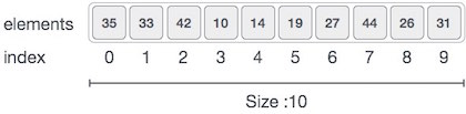
As per the above illustration, following are the important points to be considered.
Index starts with 0.
Array length is 10 which means it can store 10 elements.
Each element can be accessed via its index. For example, we can fetch an element at index 6 as 9.
Basic Operations
Following are the basic operations supported by an array.
Traverse − print all the array elements one by one.
Insertion − Adds an element at the given index.
Deletion − Deletes an element at the given index.
Search − Searches an element using the given index or by the value.
Update − Updates an element at the given index.
In C, when an array is initialized with size, then it assigns defaults values to its elements in following order.
| Data Type | Default Value |
|---|---|
| bool | false |
| char | 0 |
| int | 0 |
| float | 0.0 |
| double | 0.0f |
| void | |
| wchar_t | 0 |
Insertion Operation
Insert operation is to insert one or more data elements into an array. Based on the requirement, a new element can be added at the beginning, end, or any given index of array.
Here, we see a practical implementation of insertion operation, where we add data at the end of the array −
Algorithm
Let Array be a linear unordered array of MAX elements.
Example
Result
Let LA be a Linear Array (unordered) with N elements and K is a positive integer such that K<=N. Following is the algorithm where ITEM is inserted into the Kth position of LA −
1. Start
2. Set J = N
3. Set N = N+1
4. Repeat steps 5 and 6 while J >= K
5. Set LA[J+1] = LA[J]
6. Set J = J-1
7. Set LA[K] = ITEM
8. Stop
Example
Following is the implementation of the above algorithm −
Live Demo
#include <stdio.h>

main() {
   int LA[] = {1,3,5,7,8};
   int item = 10, k = 3, n = 5;
   int i = 0, j = n;

   printf("The original array elements are :\n");

   for(i = 0; i<n; i++) {
      printf("LA[%d] = %d \n", i, LA[i]);
   }

   n = n + 1;

   while( j >= k) {
      LA[j+1] = LA[j];
      j = j - 1;
   }

   LA[k] = item;

   printf("The array elements after insertion :\n");

   for(i = 0; i<n; i++) {
      printf("LA[%d] = %d \n", i, LA[i]);
   }
}
When we compile and execute the above program, it produces the following result −
Output
The original array elements are :
LA[0] = 1
LA[1] = 3
LA[2] = 5
LA[3] = 7
LA[4] = 8
The array elements after insertion :
LA[0] = 1
LA[1] = 3
LA[2] = 5
LA[3] = 10
LA[4] = 7
LA[5] = 8
For other variations of array insertion operation click here
Deletion Operation
Deletion refers to removing an existing element from the array and re-organizing all elements of an array.
Algorithm
Consider LA is a linear array with N elements and K is a positive integer such that K<=N. Following is the algorithm to delete an element available at the Kth position of LA.
1. Start
2. Set J = K
3. Repeat steps 4 and 5 while J < N
4. Set LA[J] = LA[J + 1]
5. Set J = J+1
6. Set N = N-1
7. Stop
Example
Following is the implementation of the above algorithm −
Live Demo
#include <stdio.h>

void main() {
   int LA[] = {1,3,5,7,8};
   int k = 3, n = 5;
   int i, j;

   printf("The original array elements are :\n");

   for(i = 0; i<n; i++) {
      printf("LA[%d] = %d \n", i, LA[i]);
   }

   j = k;

   while( j < n) {
      LA[j-1] = LA[j];
      j = j + 1;
   }

   n = n -1;

   printf("The array elements after deletion :\n");

   for(i = 0; i<n; i++) {
      printf("LA[%d] = %d \n", i, LA[i]);
   }
}
When we compile and execute the above program, it produces the following result −
Output
The original array elements are :
LA[0] = 1
LA[1] = 3
LA[2] = 5
LA[3] = 7
LA[4] = 8
The array elements after deletion :
LA[0] = 1
LA[1] = 3
LA[2] = 7
LA[3] = 8
Search Operation
You can perform a search for an array element based on its value or its index.
Algorithm
Consider LA is a linear array with N elements and K is a positive integer such that K<=N. Following is the algorithm to find an element with a value of ITEM using sequential search.
1. Start
2. Set J = 0
3. Repeat steps 4 and 5 while J < N
4. IF LA[J] is equal ITEM THEN GOTO STEP 6
5. Set J = J +1
6. PRINT J, ITEM
7. Stop
Example
Following is the implementation of the above algorithm −
Live Demo
#include <stdio.h>

void main() {
   int LA[] = {1,3,5,7,8};
   int item = 5, n = 5;
   int i = 0, j = 0;

   printf("The original array elements are :\n");

   for(i = 0; i<n; i++) {
      printf("LA[%d] = %d \n", i, LA[i]);
   }

   while( j < n){
      if( LA[j] == item ) {
         break;
      }

      j = j + 1;
   }

   printf("Found element %d at position %d\n", item, j+1);
}
When we compile and execute the above program, it produces the following result −
Output
The original array elements are :
LA[0] = 1
LA[1] = 3
LA[2] = 5
LA[3] = 7
LA[4] = 8
Found element 5 at position 3
Update Operation
Update operation refers to updating an existing element from the array at a given index.
Algorithm
Consider LA is a linear array with N elements and K is a positive integer such that K<=N. Following is the algorithm to update an element available at the Kth position of LA.
1. Start
2. Set LA[K-1] = ITEM
3. Stop
Example
Following is the implementation of the above algorithm −
Live Demo
#include <stdio.h>

void main() {
   int LA[] = {1,3,5,7,8};
   int k = 3, n = 5, item = 10;
   int i, j;

   printf("The original array elements are :\n");

   for(i = 0; i<n; i++) {
      printf("LA[%d] = %d \n", i, LA[i]);
   }

   LA[k-1] = item;

   printf("The array elements after updation :\n");

   for(i = 0; i<n; i++) {
      printf("LA[%d] = %d \n", i, LA[i]);
   }
}
When we compile and execute the above program, it produces the following result −
Output
The original array elements are :
LA[0] = 1
LA[1] = 3
LA[2] = 5
LA[3] = 7
LA[4] = 8
The array elements after updation :
LA[0] = 1
LA[1] = 3
LA[2] = 10
LA[3] = 7
LA[4] = 8
Data Structure and Algorithms - Linked List
A linked list is a sequence of data structures, which are connected together via links.
Linked List is a sequence of links which contains items. Each link contains a connection to another link. Linked list is the second most-used data structure after array. Following are the important terms to understand the concept of Linked List.
Link − Each link of a linked list can store a data called an element.
Next − Each link of a linked list contains a link to the next link called Next.
LinkedList − A Linked List contains the connection link to the first link called First.
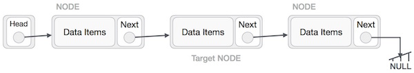
Linked List Representation
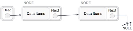
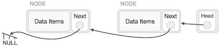
Linked list can be visualized as a chain of nodes, where every node points to the next node.
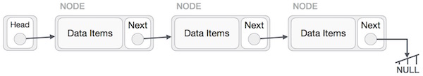
As per the above illustration, following are the important points to be considered.
Linked List contains a link element called first.
Each link carries a data field(s) and a link field called next.
Each link is linked with its next link using its next link.
Last link carries a link as null to mark the end of the list.
Types of Linked List
Following are the various types of linked list.
Simple Linked List − Item navigation is forward only.
Doubly Linked List − Items can be navigated forward and backward.
Circular Linked List − Last item contains link of the first element as next and the first element has a link to the last element as previous.
Basic Operations
Following are the basic operations supported by a list.
Insertion − Adds an element at the beginning of the list.
Deletion − Deletes an element at the beginning of the list.
Display − Displays the complete list.
Search − Searches an element using the given key.
Delete − Deletes an element using the given key.
Insertion Operation
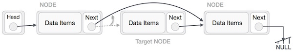
Adding a new node in linked list is a more than one step activity. We shall learn this with diagrams here. First, create a node using the same structure and find the location where it has to be inserted.
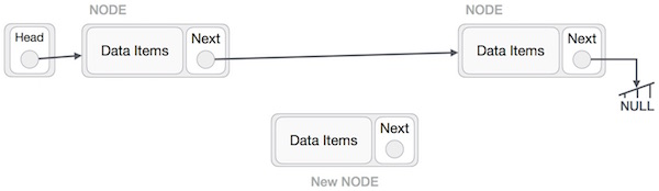
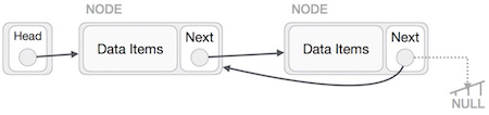
Imagine that we are inserting a node B (NewNode), between A (LeftNode) and C (RightNode). Then point B.next to C −
NewNode.next −> RightNode;
It should look like this −
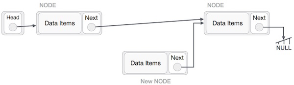
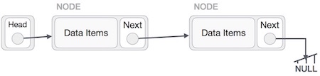
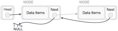
Now, the next node at the left should point to the new node.
LeftNode.next −> NewNode;
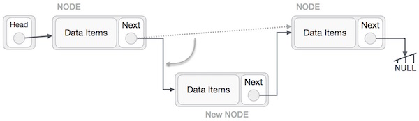
This will put the new node in the middle of the two. The new list should look like this −
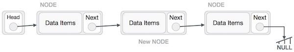
Similar steps should be taken if the node is being inserted at the beginning of the list. While inserting it at the end, the second last node of the list should point to the new node and the new node will point to NULL.
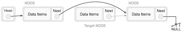
Deletion Operation
Deletion is also a more than one step process. We shall learn with pictorial representation. First, locate the target node to be removed, by using searching algorithms.
The left (previous) node of the target node now should point to the next node of the target node −
LeftNode.next −> TargetNode.next;
This will remove the link that was pointing to the target node. Now, using the following code, we will remove what the target node is pointing at.
TargetNode.next −> NULL;
We need to use the deleted node. We can keep that in memory otherwise we can simply deallocate memory and wipe off the target node completely.
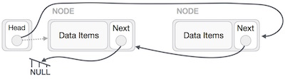
Reverse Operation
This operation is a thorough one. We need to make the last node to be pointed by the head node and reverse the whole linked list.
First, we traverse to the end of the list. It should be pointing to NULL. Now, we shall make it point to its previous node −
We have to make sure that the last node is not the lost node. So we'll have some temp node, which looks like the head node pointing to the last node. Now, we shall make all left side nodes point to their previous nodes one by one.
Except the node (first node) pointed by the head node, all nodes should point to their predecessor, making them their new successor. The first node will point to NULL.
We'll make the head node point to the new first node by using the temp node.
The linked list is now reversed. To see linked list implementation in C programming language, please click here.
Data Structure - Doubly Linked List
Doubly Linked List is a variation of Linked list in which navigation is possible in both ways, either forward and backward easily as compared to Single Linked List. Following are the important terms to understand the concept of doubly linked list.
Link − Each link of a linked list can store a data called an element.
Next − Each link of a linked list contains a link to the next link called Next.
Prev − Each link of a linked list contains a link to the previous link called Prev.
LinkedList − A Linked List contains the connection link to the first link called First and to the last link called Last.
Doubly Linked List Representation
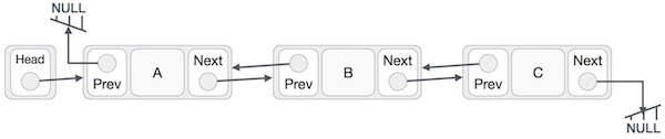
As per the above illustration, following are the important points to be considered.
Doubly Linked List contains a link element called first and last.
Each link carries a data field(s) and two link fields called next and prev.
Each link is linked with its next link using its next link.
Each link is linked with its previous link using its previous link.
The last link carries a link as null to mark the end of the list.
Basic Operations
Following are the basic operations supported by a list.
Insertion − Adds an element at the beginning of the list.
Deletion − Deletes an element at the beginning of the list.
Insert Last − Adds an element at the end of the list.
Delete Last − Deletes an element from the end of the list.
Insert After − Adds an element after an item of the list.
Delete − Deletes an element from the list using the key.
Display forward − Displays the complete list in a forward manner.
Display backward − Displays the complete list in a backward manner.
Insertion Operation
Following code demonstrates the insertion operation at the beginning of a doubly linked list.
Example
//insert link at the first location
void insertFirst(int key, int data) {

   //create a link
   struct node *link = (struct node*) malloc(sizeof(struct node));
   link->key = key;
   link->data = data;

   if(isEmpty()) {
      //make it the last link
      last = link;
   } else {
      //update first prev link
      head->prev = link;
   }

   //point it to old first link
   link->next = head;

   //point first to new first link
   head = link;
}
Deletion Operation
Following code demonstrates the deletion operation at the beginning of a doubly linked list.
Example
//delete first item
struct node* deleteFirst() {

   //save reference to first link
   struct node *tempLink = head;

   //if only one link
   if(head->next == NULL) {
      last = NULL;
   } else {
      head->next->prev = NULL;
   }

   head = head->next;

   //return the deleted link
   return tempLink;
}
Insertion at the End of an Operation
Following code demonstrates the insertion operation at the last position of a doubly linked list.
Example
//insert link at the last location
void insertLast(int key, int data) {

   //create a link
   struct node *link = (struct node*) malloc(sizeof(struct node));
   link->key = key;
   link->data = data;

   if(isEmpty()) {
      //make it the last link
      last = link;
   } else {
      //make link a new last link
      last->next = link;

      //mark old last node as prev of new link
      link->prev = last;
   }

   //point last to new last node
   last = link;
}
To see the implementation in C programming language, please click here.
Data Structure - Circular Linked List
Circular Linked List is a variation of Linked list in which the first element points to the last element and the last element points to the first element. Both Singly Linked List and Doubly Linked List can be made into a circular linked list.
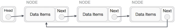
Singly Linked List as Circular
In singly linked list, the next pointer of the last node points to the first node.
Doubly Linked List as Circular
In doubly linked list, the next pointer of the last node points to the first node and the previous pointer of the first node points to the last node making the circular in both directions.
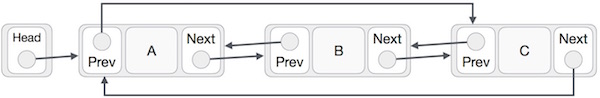
As per the above illustration, following are the important points to be considered.
The last link's next points to the first link of the list in both cases of singly as well as doubly linked list.
The first link's previous points to the last of the list in case of doubly linked list.
Basic Operations
Following are the important operations supported by a circular list.
insert − Inserts an element at the start of the list.
delete − Deletes an element from the start of the list.
display − Displays the list.
Insertion Operation
Following code demonstrates the insertion operation in a circular linked list based on single linked list.
Example
//insert link at the first location
void insertFirst(int key, int data) {
   //create a link
   struct node *link = (struct node*) malloc(sizeof(struct node));
   link->key = key;
   link->data= data;

   if (isEmpty()) {
      head = link;
      head->next = head;
   } else {
      //point it to old first node
      link->next = head;

      //point first to new first node
      head = link;
   }
}
Deletion Operation
Following code demonstrates the deletion operation in a circular linked list based on single linked list.
//delete first item
struct node * deleteFirst() {
   //save reference to first link
   struct node *tempLink = head;

   if(head->next == head) {
      head = NULL;
      return tempLink;
   }

   //mark next to first link as first
   head = head->next;

   //return the deleted link
   return tempLink;
}
Display List Operation
Following code demonstrates the display list operation in a circular linked list.
//display the list
void printList() {
   struct node *ptr = head;
   printf("\n[ ");

   //start from the beginning
   if(head != NULL) {
      while(ptr->next != ptr) {
         printf("(%d,%d) ",ptr->key,ptr->data);
         ptr = ptr->next;
      }
   }

   printf(" ]");
}
To know about its implementation in C programming language, please click here.
Data Structure and Algorithms - Stack
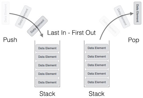
A stack is an Abstract Data Type (ADT), commonly used in most programming languages. It is named stack as it behaves like a real-world stack, for example – a deck of cards or a pile of plates, etc.

A real-world stack allows operations at one end only. For example, we can place or remove a card or plate from the top of the stack only. Likewise, Stack ADT allows all data operations at one end only. At any given time, we can only access the top element of a stack.
This feature makes it LIFO data structure. LIFO stands for Last-in-first-out. Here, the element which is placed (inserted or added) last, is accessed first. In stack terminology, insertion operation is called PUSH operation and removal operation is called POP operation.
Stack Representation
The following diagram depicts a stack and its operations −
A stack can be implemented by means of Array, Structure, Pointer, and Linked List. Stack can either be a fixed size one or it may have a sense of dynamic resizing. Here, we are going to implement stack using arrays, which makes it a fixed size stack implementation.
Basic Operations
Stack operations may involve initializing the stack, using it and then de-initializing it. Apart from these basic stuffs, a stack is used for the following two primary operations −
push() − Pushing (storing) an element on the stack.
pop() − Removing (accessing) an element from the stack.
When data is PUSHed onto stack.
To use a stack efficiently, we need to check the status of stack as well. For the same purpose, the following functionality is added to stacks −
peek() − get the top data element of the stack, without removing it.
isFull() − check if stack is full.
isEmpty() − check if stack is empty.
At all times, we maintain a pointer to the last PUSHed data on the stack. As this pointer always represents the top of the stack, hence named top. The top pointer provides top value of the stack without actually removing it.
First we should learn about procedures to support stack functions −
peek()
Algorithm of peek() function −
begin procedure peek
   return stack[top]
end procedure
Implementation of peek() function in C programming language −
Example
int peek() {
   return stack[top];
}
isfull()
Algorithm of isfull() function −
begin procedure isfull

   if top equals to MAXSIZE
      return true
   else
      return false
   endif

end procedure
Implementation of isfull() function in C programming language −
Example
bool isfull() {
   if(top == MAXSIZE)
      return true;
   else
      return false;
}
isempty()
Algorithm of isempty() function −
begin procedure isempty

   if top less than 1
      return true
   else
      return false
   endif

end procedure
Implementation of isempty() function in C programming language is slightly different. We initialize top at -1, as the index in array starts from 0. So we check if the top is below zero or -1 to determine if the stack is empty. Here's the code −
Example
bool isempty() {
   if(top == -1)
      return true;
   else
      return false;
}
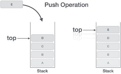
Push Operation
The process of putting a new data element onto stack is known as a Push Operation. Push operation involves a series of steps −
Step 1 − Checks if the stack is full.
Step 2 − If the stack is full, produces an error and exit.
Step 3 − If the stack is not full, increments top to point next empty space.
Step 4 − Adds data element to the stack location, where top is pointing.
Step 5 − Returns success.
If the linked list is used to implement the stack, then in step 3, we need to allocate space dynamically.
Algorithm for PUSH Operation
A simple algorithm for Push operation can be derived as follows −
begin procedure push: stack, data

   if stack is full
      return null
   endif

   top ← top + 1
   stack[top] ← data

end procedure
Implementation of this algorithm in C, is very easy. See the following code −
Example
void push(int data) {
   if(!isFull()) {
      top = top + 1;
      stack[top] = data;
   } else {
      printf("Could not insert data, Stack is full.\n");
   }
}
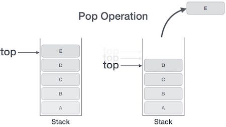
Pop Operation
Accessing the content while removing it from the stack, is known as a Pop Operation. In an array implementation of pop() operation, the data element is not actually removed, instead top is decremented to a lower position in the stack to point to the next value. But in linked-list implementation, pop() actually removes data element and deallocates memory space.
A Pop operation may involve the following steps −
Step 1 − Checks if the stack is empty.
Step 2 − If the stack is empty, produces an error and exit.
Step 3 − If the stack is not empty, accesses the data element at which top is pointing.
Step 4 − Decreases the value of top by 1.
Step 5 − Returns success.
Algorithm for Pop Operation
A simple algorithm for Pop operation can be derived as follows −
begin procedure pop: stack

   if stack is empty
      return null
   endif

   data ← stack[top]
   top ← top - 1
   return data

end procedure
Implementation of this algorithm in C, is as follows −
Example
int pop(int data) {

   if(!isempty()) {
      data = stack[top];
      top = top - 1;
      return data;
   } else {
      printf("Could not retrieve data, Stack is empty.\n");
   }
}
For a complete stack program in C programming language, please click here.
Data Structure - Expression Parsing
The way to write arithmetic expression is known as a notation. An arithmetic expression can be written in three different but equivalent notations, i.e., without changing the essence or output of an expression. These notations are −
- Infix Notation
- Prefix (Polish) Notation
- Postfix (Reverse-Polish) Notation
These notations are named as how they use operator in expression. We shall learn the same here in this chapter.
Infix Notation
We write expression in infix notation, e.g. a - b + c, where operators are used in-between operands. It is easy for us humans to read, write, and speak in infix notation but the same does not go well with computing devices. An algorithm to process infix notation could be difficult and costly in terms of time and space consumption.
Prefix Notation
In this notation, operator is prefixed to operands, i.e. operator is written ahead of operands. For example, +ab. This is equivalent to its infix notation a + b. Prefix notation is also known as Polish Notation.
Postfix Notation
This notation style is known as Reversed Polish Notation. In this notation style, the operator is postfixed to the operands i.e., the operator is written after the operands. For example, ab+. This is equivalent to its infix notation a + b.
The following table briefly tries to show the difference in all three notations −
| Sr.No. | Infix Notation | Prefix Notation | Postfix Notation |
|---|---|---|---|
| 1 | a + b | + a b | a b + |
| 2 | (a + b) ∗ c | ∗ + a b c | a b + c ∗ |
| 3 | a ∗ (b + c) | ∗ a + b c | a b c + ∗ |
| 4 | a / b + c / d | + / a b / c d | a b / c d / + |
| 5 | (a + b) ∗ (c + d) | ∗ + a b + c d | a b + c d + ∗ |
| 6 | ((a + b) ∗ c) - d | - ∗ + a b c d | a b + c ∗ d - |
Parsing Expressions
As we have discussed, it is not a very efficient way to design an algorithm or program to parse infix notations. Instead, these infix notations are first converted into either postfix or prefix notations and then computed.
To parse any arithmetic expression, we need to take care of operator precedence and associativity also.
Precedence
When an operand is in between two different operators, which operator will take the operand first, is decided by the precedence of an operator over others. For example −
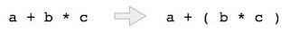
As multiplication operation has precedence over addition, b * c will be evaluated first. A table of operator precedence is provided later.
Associativity
Associativity describes the rule where operators with the same precedence appear in an expression. For example, in expression a + b − c, both + and – have the same precedence, then which part of the expression will be evaluated first, is determined by associativity of those operators. Here, both + and − are left associative, so the expression will be evaluated as (a + b) − c.
Precedence and associativity determines the order of evaluation of an expression. Following is an operator precedence and associativity table (highest to lowest) −
| Sr.No. | Operator | Precedence | Associativity |
|---|---|---|---|
| 1 | Exponentiation ^ | Highest | Right Associative |
| 2 | Multiplication ( ∗ ) & Division ( / ) | Second Highest | Left Associative |
| 3 | Addition ( + ) & Subtraction ( − ) | Lowest | Left Associative |
The above table shows the default behavior of operators. At any point of time in expression evaluation, the order can be altered by using parenthesis. For example −
In a + b*c, the expression part b*c will be evaluated first, with multiplication as precedence over addition. We here use parenthesis for a + b to be evaluated first, like (a + b)*c.
Postfix Evaluation Algorithm
We shall now look at the algorithm on how to evaluate postfix notation −
Step 1 − scan the expression from left to right
Step 2 − if it is an operand push it to stack
Step 3 − if it is an operator pull operand from stack and perform operation
Step 4 − store the output of step 3, back to stack
Step 5 − scan the expression until all operands are consumed
Step 6 − pop the stack and perform operation
To see the implementation in C programming language, please click here.
Data Structure and Algorithms - Queue
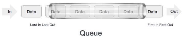
Queue is an abstract data structure, somewhat similar to Stacks. Unlike stacks, a queue is open at both its ends. One end is always used to insert data (enqueue) and the other is used to remove data (dequeue). Queue follows First-In-First-Out methodology, i.e., the data item stored first will be accessed first.

A real-world example of queue can be a single-lane one-way road, where the vehicle enters first, exits first. More real-world examples can be seen as queues at the ticket windows and bus-stops.
Queue Representation
As we now understand that in queue, we access both ends for different reasons. The following diagram given below tries to explain queue representation as data structure −
As in stacks, a queue can also be implemented using Arrays, Linked-lists, Pointers and Structures. For the sake of simplicity, we shall implement queues using one-dimensional array.
Basic Operations
Queue operations may involve initializing or defining the queue, utilizing it, and then completely erasing it from the memory. Here we shall try to understand the basic operations associated with queues −
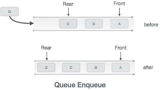
enqueue() − add (store) an item to the queue.
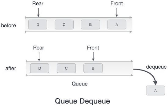
dequeue() − remove (access) an item from the queue.
Few more functions are required to make the above-mentioned queue operation efficient. These are −
peek() − Gets the element at the front of the queue without removing it.
isfull() − Checks if the queue is full.
isempty() − Checks if the queue is empty.
In queue, we always dequeue (or access) data, pointed by front pointer and while enqueing (or storing) data in the queue we take help of rear pointer.
Let's first learn about supportive functions of a queue −
peek()
This function helps to see the data at the front of the queue. The algorithm of peek() function is as follows −
Algorithm
begin procedure peek
   return queue[front]
end procedure
Implementation of peek() function in C programming language −
Example
int peek() {
   return queue[front];
}
isfull()
As we are using single dimension array to implement queue, we just check for the rear pointer to reach at MAXSIZE to determine that the queue is full. In case we maintain the queue in a circular linked-list, the algorithm will differ. Algorithm of isfull() function −
Algorithm
begin procedure isfull

   if rear equals to MAXSIZE
      return true
   else
      return false
   endif

end procedure
Implementation of isfull() function in C programming language −
Example
bool isfull() {
   if(rear == MAXSIZE - 1)
      return true;
   else
      return false;
}
isempty()
Algorithm of isempty() function −
Algorithm
begin procedure isempty

   if front is less than MIN  OR front is greater than rear
      return true
   else
      return false
   endif

end procedure
If the value of front is less than MIN or 0, it tells that the queue is not yet initialized, hence empty.
Here's the C programming code −
Example
bool isempty() {
   if(front < 0 || front > rear)
      return true;
   else
      return false;
}
Enqueue Operation
Queues maintain two data pointers, front and rear. Therefore, its operations are comparatively difficult to implement than that of stacks.
The following steps should be taken to enqueue (insert) data into a queue −
Step 1 − Check if the queue is full.
Step 2 − If the queue is full, produce overflow error and exit.
Step 3 − If the queue is not full, increment rear pointer to point the next empty space.
Step 4 − Add data element to the queue location, where the rear is pointing.
Step 5 − return success.
Sometimes, we also check to see if a queue is initialized or not, to handle any unforeseen situations.
Algorithm for enqueue operation
procedure enqueue(data)

   if queue is full
      return overflow
   endif

   rear ← rear + 1
   queue[rear] ← data
   return true

end procedure
Implementation of enqueue() in C programming language −
Example
int enqueue(int data)
   if(isfull())
      return 0;

   rear = rear + 1;
   queue[rear] = data;

   return 1;
end procedure
Dequeue Operation
Accessing data from the queue is a process of two tasks − access the data where front is pointing and remove the data after access. The following steps are taken to perform dequeue operation −
Step 1 − Check if the queue is empty.
Step 2 − If the queue is empty, produce underflow error and exit.
Step 3 − If the queue is not empty, access the data where front is pointing.
Step 4 − Increment front pointer to point to the next available data element.
Step 5 − Return success.
Algorithm for dequeue operation
procedure dequeue

   if queue is empty
      return underflow
   end if

   data = queue[front]
   front ← front + 1
   return true

end procedure
Implementation of dequeue() in C programming language −
Example
int dequeue() {
   if(isempty())
      return 0;

   int data = queue[front];
   front = front + 1;

   return data;
}
For a complete Queue program in C programming language, please click here.
Data Structure and Algorithms Linear Search
Linear search is a very simple search algorithm. In this type of search, a sequential search is made over all items one by one. Every item is checked and if a match is found then that particular item is returned, otherwise the search continues till the end of the data collection.
Algorithm
Linear Search ( Array A, Value x)

Step 1: Set i to 1
Step 2: if i > n then go to step 7
Step 3: if A[i] = x then go to step 6
Step 4: Set i to i + 1
Step 5: Go to Step 2
Step 6: Print Element x Found at index i and go to step 8
Step 7: Print element not found
Step 8: Exit
Pseudocode
procedure linear_search (list, value)

   for each item in the list
      if match item == value
         return the item's location
      end if
   end for

end procedure
To know about linear search implementation in C programming language, please click-here.
Data Structure and Algorithms Binary Search
Binary search is a fast search algorithm with run-time complexity of Ο(log n). This search algorithm works on the principle of divide and conquer. For this algorithm to work properly, the data collection should be in the sorted form.
Binary search looks for a particular item by comparing the middle most item of the collection. If a match occurs, then the index of item is returned. If the middle item is greater than the item, then the item is searched in the sub-array to the left of the middle item. Otherwise, the item is searched for in the sub-array to the right of the middle item. This process continues on the sub-array as well until the size of the subarray reduces to zero.
How Binary Search Works?
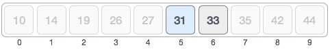
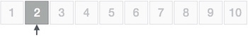
For a binary search to work, it is mandatory for the target array to be sorted. We shall learn the process of binary search with a pictorial example. The following is our sorted array and let us assume that we need to search the location of value 31 using binary search.
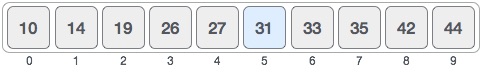
First, we shall determine half of the array by using this formula −
mid = low + (high - low) / 2
Here it is, 0 + (9 - 0 ) / 2 = 4 (integer value of 4.5). So, 4 is the mid of the array.
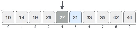
Now we compare the value stored at location 4, with the value being searched, i.e. 31. We find that the value at location 4 is 27, which is not a match. As the value is greater than 27 and we have a sorted array, so we also know that the target value must be in the upper portion of the array.
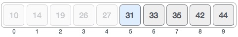
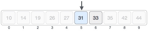
We change our low to mid + 1 and find the new mid value again.
low = mid + 1
mid = low + (high - low) / 2
Our new mid is 7 now. We compare the value stored at location 7 with our target value 31.
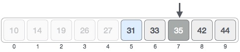
The value stored at location 7 is not a match, rather it is more than what we are looking for. So, the value must be in the lower part from this location.
Hence, we calculate the mid again. This time it is 5.
We compare the value stored at location 5 with our target value. We find that it is a match.
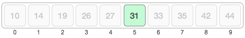
We conclude that the target value 31 is stored at location 5.
Binary search halves the searchable items and thus reduces the count of comparisons to be made to very less numbers.
Pseudocode
The pseudocode of binary search algorithms should look like this −
Procedure binary_search
   A ← sorted array
   n ← size of array
   x ← value to be searched

   Set lowerBound = 1
   Set upperBound = n

   while x not found
      if upperBound < lowerBound
         EXIT: x does not exists.

      set midPoint = lowerBound + ( upperBound - lowerBound ) / 2

      if A[midPoint] < x
         set lowerBound = midPoint + 1

      if A[midPoint] > x
         set upperBound = midPoint - 1

      if A[midPoint] = x
         EXIT: x found at location midPoint
   end while

end procedure
To know about binary search implementation using array in C programming language, please click here.
Data Structure - Interpolation Search
Interpolation search is an improved variant of binary search. This search algorithm works on the probing position of the required value. For this algorithm to work properly, the data collection should be in a sorted form and equally distributed.
Binary search has a huge advantage of time complexity over linear search. Linear search has worst-case complexity of Ο(n) whereas binary search has Ο(log n).
There are cases where the location of target data may be known in advance. For example, in case of a telephone directory, if we want to search the telephone number of Morphius. Here, linear search and even binary search will seem slow as we can directly jump to memory space where the names start from 'M' are stored.
Positioning in Binary Search
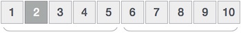
In binary search, if the desired data is not found then the rest of the list is divided in two parts, lower and higher. The search is carried out in either of them.
Even when the data is sorted, binary search does not take advantage to probe the position of the desired data.
Position Probing in Interpolation Search
Interpolation search finds a particular item by computing the probe position. Initially, the probe position is the position of the middle most item of the collection.
If a match occurs, then the index of the item is returned. To split the list into two parts, we use the following method −
mid = Lo + ((Hi - Lo) / (A[Hi] - A[Lo])) * (X - A[Lo])

where −
   A    = list
   Lo   = Lowest index of the list
   Hi   = Highest index of the list
   A[n] = Value stored at index n in the list
If the middle item is greater than the item, then the probe position is again calculated in the sub-array to the right of the middle item. Otherwise, the item is searched in the subarray to the left of the middle item. This process continues on the sub-array as well until the size of subarray reduces to zero.
Runtime complexity of interpolation search algorithm is Ο(log (log n)) as compared to Ο(log n) of BST in favorable situations.
Algorithm
As it is an improvisation of the existing BST algorithm, we are mentioning the steps to search the 'target' data value index, using position probing −
Step 1 − Start searching data from middle of the list.
Step 2 − If it is a match, return the index of the item, and exit.
Step 3 − If it is not a match, probe position.
Step 4 − Divide the list using probing formula and find the new midle.
Step 5 − If data is greater than middle, search in higher sub-list.
Step 6 − If data is smaller than middle, search in lower sub-list.
Step 7 − Repeat until match.
Pseudocode
A → Array list
N → Size of A
X → Target Value

Procedure Interpolation_Search()

   Set Lo  →  0
   Set Mid → -1
   Set Hi  →  N-1

   While X does not match

      if Lo equals to Hi OR A[Lo] equals to A[Hi]
         EXIT: Failure, Target not found
      end if

      Set Mid = Lo + ((Hi - Lo) / (A[Hi] - A[Lo])) * (X - A[Lo])

      if A[Mid] = X
         EXIT: Success, Target found at Mid
      else
         if A[Mid] < X
            Set Lo to Mid+1
         else if A[Mid] > X
            Set Hi to Mid-1
         end if
      end if
   End While

End Procedure
To know about the implementation of interpolation search in C programming language, click here.
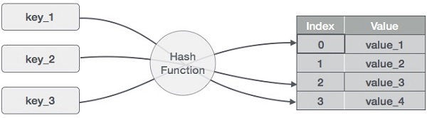
Data Structure and Algorithms - Hash Table
Hash Table is a data structure which stores data in an associative manner. In a hash table, data is stored in an array format, where each data value has its own unique index value. Access of data becomes very fast if we know the index of the desired data.
Thus, it becomes a data structure in which insertion and search operations are very fast irrespective of the size of the data. Hash Table uses an array as a storage medium and uses hash technique to generate an index where an element is to be inserted or is to be located from.
Hashing
Hashing is a technique to convert a range of key values into a range of indexes of an array. We're going to use modulo operator to get a range of key values. Consider an example of hash table of size 20, and the following items are to be stored. Item are in the (key,value) format.
- (1,20)
- (2,70)
- (42,80)
- (4,25)
- (12,44)
- (14,32)
- (17,11)
- (13,78)
- (37,98)
| Sr.No. | Key | Hash | Array Index |
|---|---|---|---|
| 1 | 1 | 1 % 20 = 1 | 1 |
| 2 | 2 | 2 % 20 = 2 | 2 |
| 3 | 42 | 42 % 20 = 2 | 2 |
| 4 | 4 | 4 % 20 = 4 | 4 |
| 5 | 12 | 12 % 20 = 12 | 12 |
| 6 | 14 | 14 % 20 = 14 | 14 |
| 7 | 17 | 17 % 20 = 17 | 17 |
| 8 | 13 | 13 % 20 = 13 | 13 |
| 9 | 37 | 37 % 20 = 17 | 17 |
Linear Probing
As we can see, it may happen that the hashing technique is used to create an already used index of the array. In such a case, we can search the next empty location in the array by looking into the next cell until we find an empty cell. This technique is called linear probing.
| Sr.No. | Key | Hash | Array Index | After Linear Probing, Array Index |
|---|---|---|---|---|
| 1 | 1 | 1 % 20 = 1 | 1 | 1 |
| 2 | 2 | 2 % 20 = 2 | 2 | 2 |
| 3 | 42 | 42 % 20 = 2 | 2 | 3 |
| 4 | 4 | 4 % 20 = 4 | 4 | 4 |
| 5 | 12 | 12 % 20 = 12 | 12 | 12 |
| 6 | 14 | 14 % 20 = 14 | 14 | 14 |
| 7 | 17 | 17 % 20 = 17 | 17 | 17 |
| 8 | 13 | 13 % 20 = 13 | 13 | 13 |
| 9 | 37 | 37 % 20 = 17 | 17 | 18 |
Basic Operations
Following are the basic primary operations of a hash table.
Search − Searches an element in a hash table.
Insert − inserts an element in a hash table.
delete − Deletes an element from a hash table.
DataItem
Define a data item having some data and key, based on which the search is to be conducted in a hash table.
struct DataItem {
   int data;
   int key;
};
Hash Method
Define a hashing method to compute the hash code of the key of the data item.
int hashCode(int key){
   return key % SIZE;
}
Search Operation
Whenever an element is to be searched, compute the hash code of the key passed and locate the element using that hash code as index in the array. Use linear probing to get the element ahead if the element is not found at the computed hash code.
Example
struct DataItem *search(int key) {
   //get the hash
   int hashIndex = hashCode(key);

   //move in array until an empty
   while(hashArray[hashIndex] != NULL) {

      if(hashArray[hashIndex]->key == key)
         return hashArray[hashIndex];

      //go to next cell
      ++hashIndex;

      //wrap around the table
      hashIndex %= SIZE;
   }

   return NULL;
}
Insert Operation
Whenever an element is to be inserted, compute the hash code of the key passed and locate the index using that hash code as an index in the array. Use linear probing for empty location, if an element is found at the computed hash code.
Example
void insert(int key,int data) {
   struct DataItem *item = (struct DataItem*) malloc(sizeof(struct DataItem));
   item->data = data;
   item->key = key;

   //get the hash
   int hashIndex = hashCode(key);

   //move in array until an empty or deleted cell
   while(hashArray[hashIndex] != NULL && hashArray[hashIndex]->key != -1) {
      //go to next cell
      ++hashIndex;

      //wrap around the table
      hashIndex %= SIZE;
   }

   hashArray[hashIndex] = item;
}
Delete Operation
Whenever an element is to be deleted, compute the hash code of the key passed and locate the index using that hash code as an index in the array. Use linear probing to get the element ahead if an element is not found at the computed hash code. When found, store a dummy item there to keep the performance of the hash table intact.
Example
struct DataItem* delete(struct DataItem* item) {
   int key = item->key;

   //get the hash
   int hashIndex = hashCode(key);

   //move in array until an empty
   while(hashArray[hashIndex] !=NULL) {

      if(hashArray[hashIndex]->key == key) {
         struct DataItem* temp = hashArray[hashIndex];

         //assign a dummy item at deleted position
         hashArray[hashIndex] = dummyItem;
         return temp;
      }

      //go to next cell
      ++hashIndex;

      //wrap around the table
      hashIndex %= SIZE;
   }

   return NULL;
}
To know about hash implementation in C programming language, please click here.
Data Structure - Sorting Techniques
Sorting refers to arranging data in a particular format. Sorting algorithm specifies the way to arrange data in a particular order. Most common orders are in numerical or lexicographical order.
The importance of sorting lies in the fact that data searching can be optimized to a very high level, if data is stored in a sorted manner. Sorting is also used to represent data in more readable formats. Following are some of the examples of sorting in real-life scenarios −
Telephone Directory − The telephone directory stores the telephone numbers of people sorted by their names, so that the names can be searched easily.
Dictionary − The dictionary stores words in an alphabetical order so that searching of any word becomes easy.
In-place Sorting and Not-in-place Sorting
Sorting algorithms may require some extra space for comparison and temporary storage of few data elements. These algorithms do not require any extra space and sorting is said to happen in-place, or for example, within the array itself. This is called in-place sorting. Bubble sort is an example of in-place sorting.
However, in some sorting algorithms, the program requires space which is more than or equal to the elements being sorted. Sorting which uses equal or more space is called not-in-place sorting. Merge-sort is an example of not-in-place sorting.
Stable and Not Stable Sorting
If a sorting algorithm, after sorting the contents, does not change the sequence of similar content in which they appear, it is called stable sorting.
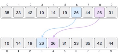
If a sorting algorithm, after sorting the contents, changes the sequence of similar content in which they appear, it is called unstable sorting.
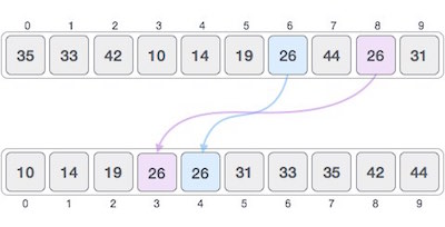
Stability of an algorithm matters when we wish to maintain the sequence of original elements, like in a tuple for example.
Adaptive and Non-Adaptive Sorting Algorithm
A sorting algorithm is said to be adaptive, if it takes advantage of already 'sorted' elements in the list that is to be sorted. That is, while sorting if the source list has some element already sorted, adaptive algorithms will take this into account and will try not to re-order them.
A non-adaptive algorithm is one which does not take into account the elements which are already sorted. They try to force every single element to be re-ordered to confirm their sortedness.
Important Terms
Some terms are generally coined while discussing sorting techniques, here is a brief introduction to them −
Increasing Order
A sequence of values is said to be in increasing order, if the successive element is greater than the previous one. For example, 1, 3, 4, 6, 8, 9 are in increasing order, as every next element is greater than the previous element.
Decreasing Order
A sequence of values is said to be in decreasing order, if the successive element is less than the current one. For example, 9, 8, 6, 4, 3, 1 are in decreasing order, as every next element is less than the previous element.
Non-Increasing Order
A sequence of values is said to be in non-increasing order, if the successive element is less than or equal to its previous element in the sequence. This order occurs when the sequence contains duplicate values. For example, 9, 8, 6, 3, 3, 1 are in non-increasing order, as every next element is less than or equal to (in case of 3) but not greater than any previous element.
Non-Decreasing Order
A sequence of values is said to be in non-decreasing order, if the successive element is greater than or equal to its previous element in the sequence. This order occurs when the sequence contains duplicate values. For example, 1, 3, 3, 6, 8, 9 are in non-decreasing order, as every next element is greater than or equal to (in case of 3) but not less than the previous one.
Data Structure - Bubble Sort Algorithm
Bubble sort is a simple sorting algorithm. This sorting algorithm is comparison-based algorithm in which each pair of adjacent elements is compared and the elements are swapped if they are not in order. This algorithm is not suitable for large data sets as its average and worst case complexity are of Ο(n2) where n is the number of items.
How Bubble Sort Works?
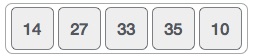
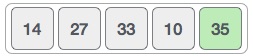
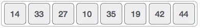
We take an unsorted array for our example. Bubble sort takes Ο(n2) time so we're keeping it short and precise.
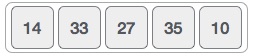
Bubble sort starts with very first two elements, comparing them to check which one is greater.
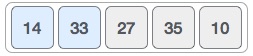
In this case, value 33 is greater than 14, so it is already in sorted locations. Next, we compare 33 with 27.
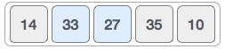
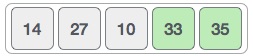
We find that 27 is smaller than 33 and these two values must be swapped.
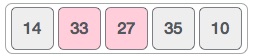
The new array should look like this −
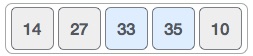
Next we compare 33 and 35. We find that both are in already sorted positions.
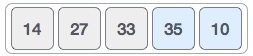
Then we move to the next two values, 35 and 10.
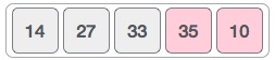
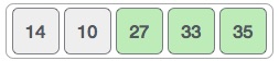
We know then that 10 is smaller 35. Hence they are not sorted.
We swap these values. We find that we have reached the end of the array. After one iteration, the array should look like this −
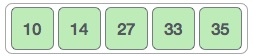
To be precise, we are now showing how an array should look like after each iteration. After the second iteration, it should look like this −
Notice that after each iteration, at least one value moves at the end.
And when there's no swap required, bubble sorts learns that an array is completely sorted.
Now we should look into some practical aspects of bubble sort.
Algorithm
We assume list is an array of n elements. We further assume that swap function swaps the values of the given array elements.
begin BubbleSort(list)

   for all elements of list
      if list[i] > list[i+1]
         swap(list[i], list[i+1])
      end if
   end for

   return list

end BubbleSort
Pseudocode
We observe in algorithm that Bubble Sort compares each pair of array element unless the whole array is completely sorted in an ascending order. This may cause a few complexity issues like what if the array needs no more swapping as all the elements are already ascending.
To ease-out the issue, we use one flag variable swapped which will help us see if any swap has happened or not. If no swap has occurred, i.e. the array requires no more processing to be sorted, it will come out of the loop.
Pseudocode of BubbleSort algorithm can be written as follows −
procedure bubbleSort( list : array of items )

   loop = list.count;

   for i = 0 to loop-1 do:
      swapped = false

      for j = 0 to loop-1 do:

         /* compare the adjacent elements */
         if list[j] > list[j+1] then
            /* swap them */
            swap( list[j], list[j+1] )
            swapped = true
         end if

      end for

      /*if no number was swapped that means
      array is sorted now, break the loop.*/

      if(not swapped) then
         break
      end if

   end for

end procedure return list
Implementation
One more issue we did not address in our original algorithm and its improvised pseudocode, is that, after every iteration the highest values settles down at the end of the array. Hence, the next iteration need not include already sorted elements. For this purpose, in our implementation, we restrict the inner loop to avoid already sorted values.
To know about bubble sort implementation in C programming language, please click here.
Data Structure and Algorithms Insertion Sort
This is an in-place comparison-based sorting algorithm. Here, a sub-list is maintained which is always sorted. For example, the lower part of an array is maintained to be sorted. An element which is to be 'insert'ed in this sorted sub-list, has to find its appropriate place and then it has to be inserted there. Hence the name, insertion sort.
The array is searched sequentially and unsorted items are moved and inserted into the sorted sub-list (in the same array). This algorithm is not suitable for large data sets as its average and worst case complexity are of Ο(n2), where n is the number of items.
How Insertion Sort Works?
We take an unsorted array for our example.
Insertion sort compares the first two elements.
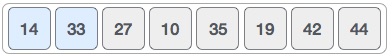
It finds that both 14 and 33 are already in ascending order. For now, 14 is in sorted sub-list.
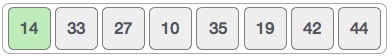
Insertion sort moves ahead and compares 33 with 27.
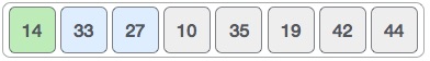
And finds that 33 is not in the correct position.
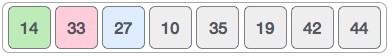
It swaps 33 with 27. It also checks with all the elements of sorted sub-list. Here we see that the sorted sub-list has only one element 14, and 27 is greater than 14. Hence, the sorted sub-list remains sorted after swapping.
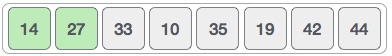
By now we have 14 and 27 in the sorted sub-list. Next, it compares 33 with 10.
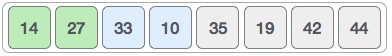
These values are not in a sorted order.
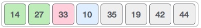
So we swap them.
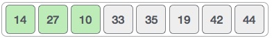
However, swapping makes 27 and 10 unsorted.
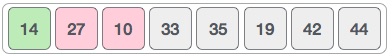
Hence, we swap them too.
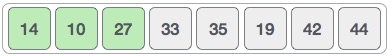
Again we find 14 and 10 in an unsorted order.
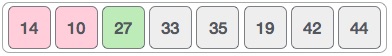
We swap them again. By the end of third iteration, we have a sorted sub-list of 4 items.
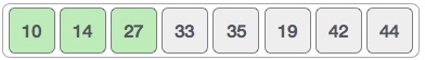
This process goes on until all the unsorted values are covered in a sorted sub-list. Now we shall see some programming aspects of insertion sort.
Algorithm
Now we have a bigger picture of how this sorting technique works, so we can derive simple steps by which we can achieve insertion sort.
Step 1 − If it is the first element, it is already sorted. return 1;
Step 2 − Pick next element
Step 3 − Compare with all elements in the sorted sub-list
Step 4 − Shift all the elements in the sorted sub-list that is greater than the
         value to be sorted
Step 5 − Insert the value
Step 6 − Repeat until list is sorted
Pseudocode
procedure insertionSort( A : array of items )
   int holePosition
   int valueToInsert

   for i = 1 to length(A) inclusive do:

      /* select value to be inserted */
      valueToInsert = A[i]
      holePosition = i

      /*locate hole position for the element to be inserted */

      while holePosition > 0 and A[holePosition-1] > valueToInsert do:
         A[holePosition] = A[holePosition-1]
         holePosition = holePosition -1
      end while

      /* insert the number at hole position */
      A[holePosition] = valueToInsert

   end for

end procedure
To know about insertion sort implementation in C programming language, please click here.
Data Structure and Algorithms Selection Sort
Selection sort is a simple sorting algorithm. This sorting algorithm is an in-place comparison-based algorithm in which the list is divided into two parts, the sorted part at the left end and the unsorted part at the right end. Initially, the sorted part is empty and the unsorted part is the entire list.
The smallest element is selected from the unsorted array and swapped with the leftmost element, and that element becomes a part of the sorted array. This process continues moving unsorted array boundary by one element to the right.
This algorithm is not suitable for large data sets as its average and worst case complexities are of Ο(n2), where n is the number of items.
How Selection Sort Works?
Consider the following depicted array as an example.
For the first position in the sorted list, the whole list is scanned sequentially. The first position where 14 is stored presently, we search the whole list and find that 10 is the lowest value.
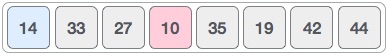
So we replace 14 with 10. After one iteration 10, which happens to be the minimum value in the list, appears in the first position of the sorted list.
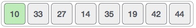
For the second position, where 33 is residing, we start scanning the rest of the list in a linear manner.
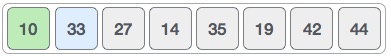
We find that 14 is the second lowest value in the list and it should appear at the second place. We swap these values.
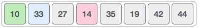
After two iterations, two least values are positioned at the beginning in a sorted manner.
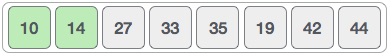
The same process is applied to the rest of the items in the array.
Following is a pictorial depiction of the entire sorting process −
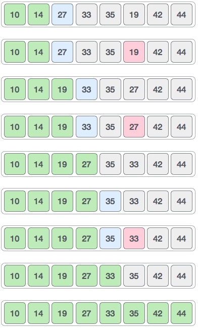
Now, let us learn some programming aspects of selection sort.
Algorithm
Step 1 − Set MIN to location 0
Step 2 − Search the minimum element in the list
Step 3 − Swap with value at location MIN
Step 4 − Increment MIN to point to next element
Step 5 − Repeat until list is sorted
Pseudocode
procedure selection sort
   list  : array of items
   n     : size of list

   for i = 1 to n - 1
   /* set current element as minimum*/
      min = i

      /* check the element to be minimum */

      for j = i+1 to n
         if list[j] < list[min] then
            min = j;
         end if
      end for

      /* swap the minimum element with the current element*/
      if indexMin != i  then
         swap list[min] and list[i]
      end if
   end for

end procedure
To know about selection sort implementation in C programming language, please click here.
Data Structures - Merge Sort Algorithm
Merge sort is a sorting technique based on divide and conquer technique. With worst-case time complexity being Ο(n log n), it is one of the most respected algorithms.
Merge sort first divides the array into equal halves and then combines them in a sorted manner.
How Merge Sort Works?
To understand merge sort, we take an unsorted array as the following −
We know that merge sort first divides the whole array iteratively into equal halves unless the atomic values are achieved. We see here that an array of 8 items is divided into two arrays of size 4.
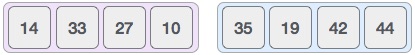
This does not change the sequence of appearance of items in the original. Now we divide these two arrays into halves.
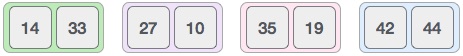
We further divide these arrays and we achieve atomic value which can no more be divided.

Now, we combine them in exactly the same manner as they were broken down. Please note the color codes given to these lists.
We first compare the element for each list and then combine them into another list in a sorted manner. We see that 14 and 33 are in sorted positions. We compare 27 and 10 and in the target list of 2 values we put 10 first, followed by 27. We change the order of 19 and 35 whereas 42 and 44 are placed sequentially.
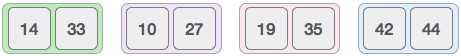
In the next iteration of the combining phase, we compare lists of two data values, and merge them into a list of found data values placing all in a sorted order.
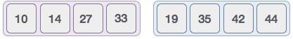
After the final merging, the list should look like this −
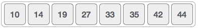
Now we should learn some programming aspects of merge sorting.
Algorithm
Merge sort keeps on dividing the list into equal halves until it can no more be divided. By definition, if it is only one element in the list, it is sorted. Then, merge sort combines the smaller sorted lists keeping the new list sorted too.
Step 1 − if it is only one element in the list it is already sorted, return.
Step 2 − divide the list recursively into two halves until it can no more be divided.
Step 3 − merge the smaller lists into new list in sorted order.
Pseudocode
We shall now see the pseudocodes for merge sort functions. As our algorithms point out two main functions − divide & merge.
Merge sort works with recursion and we shall see our implementation in the same way.
procedure mergesort( var a as array )
   if ( n == 1 ) return a

   var l1 as array = a[0] ... a[n/2]
   var l2 as array = a[n/2+1] ... a[n]

   l1 = mergesort( l1 )
   l2 = mergesort( l2 )

   return merge( l1, l2 )
end procedure

procedure merge( var a as array, var b as array )

   var c as array
   while ( a and b have elements )
      if ( a[0] > b[0] )
         add b[0] to the end of c
         remove b[0] from b
      else
         add a[0] to the end of c
         remove a[0] from a
      end if
   end while

   while ( a has elements )
      add a[0] to the end of c
      remove a[0] from a
   end while

   while ( b has elements )
      add b[0] to the end of c
      remove b[0] from b
   end while

   return c

end procedure
To know about merge sort implementation in C programming language, please click here.
Shell sort is a highly efficient sorting algorithm and is based on insertion sort algorithm. This algorithm avoids large shifts as in case of insertion sort, if the smaller value is to the far right and has to be moved to the far left.
This algorithm uses insertion sort on a widely spread elements, first to sort them and then sorts the less widely spaced elements. This spacing is termed as interval. This interval is calculated based on Knuth's formula as −
Knuth's Formula
h = h * 3 + 1
where −
   h is interval with initial value 1
This algorithm is quite efficient for medium-sized data sets as its average and worst case complexity are of Ο(n), where n is the number of items.
How Shell Sort Works?
Let us consider the following example to have an idea of how shell sort works. We take the same array we have used in our previous examples. For our example and ease of understanding, we take the interval of 4. Make a virtual sub-list of all values located at the interval of 4 positions. Here these values are {35, 14}, {33, 19}, {42, 27} and {10, 44}
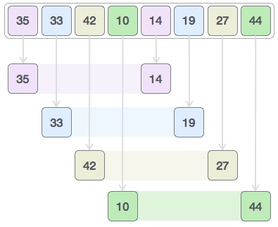
We compare values in each sub-list and swap them (if necessary) in the original array. After this step, the new array should look like this −
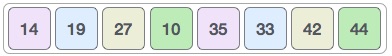
Then, we take interval of 2 and this gap generates two sub-lists - {14, 27, 35, 42}, {19, 10, 33, 44}
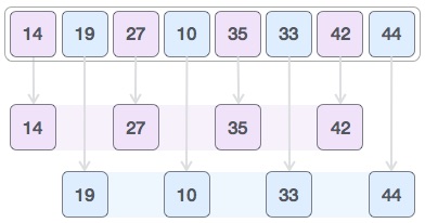
We compare and swap the values, if required, in the original array. After this step, the array should look like this −
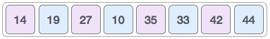
Finally, we sort the rest of the array using interval of value 1. Shell sort uses insertion sort to sort the array.
Following is the step-by-step depiction −
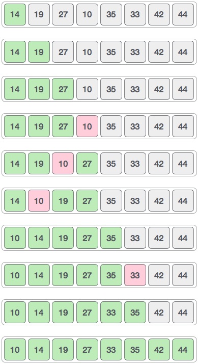
We see that it required only four swaps to sort the rest of the array.
Algorithm
Following is the algorithm for shell sort.
Step 1 − Initialize the value of h
Step 2 − Divide the list into smaller sub-list of equal interval h
Step 3 − Sort these sub-lists using insertion sort
Step 3 − Repeat until complete list is sorted
Pseudocode
Following is the pseudocode for shell sort.
procedure shellSort()
   A : array of items

   /* calculate interval*/
   while interval < A.length /3 do:
      interval = interval * 3 + 1
   end while

   while interval > 0 do:

      for outer = interval; outer < A.length; outer ++ do:

      /* select value to be inserted */
      valueToInsert = A[outer]
      inner = outer;

         /*shift element towards right*/
         while inner > interval -1 && A[inner - interval] >= valueToInsert do:
            A[inner] = A[inner - interval]
            inner = inner - interval
         end while

      /* insert the number at hole position */
      A[inner] = valueToInsert

      end for

   /* calculate interval*/
   interval = (interval -1) /3;

   end while

end procedure
To know about shell sort implementation in C programming language, please click here.
Data Structure and Algorithms - Shell Sort
Shell sort is a highly efficient sorting algorithm and is based on insertion sort algorithm. This algorithm avoids large shifts as in case of insertion sort, if the smaller value is to the far right and has to be moved to the far left.
This algorithm uses insertion sort on a widely spread elements, first to sort them and then sorts the less widely spaced elements. This spacing is termed as interval. This interval is calculated based on Knuth's formula as −
Knuth's Formula
h = h * 3 + 1
where −
   h is interval with initial value 1
This algorithm is quite efficient for medium-sized data sets as its average and worst-case complexity of this algorithm depends on the gap sequence the best known is Ο(n), where n is the number of items. And the worst case space complexity is O(n).
How Shell Sort Works?
Let us consider the following example to have an idea of how shell sort works. We take the same array we have used in our previous examples. For our example and ease of understanding, we take the interval of 4. Make a virtual sub-list of all values located at the interval of 4 positions. Here these values are {35, 14}, {33, 19}, {42, 27} and {10, 44}
We compare values in each sub-list and swap them (if necessary) in the original array. After this step, the new array should look like this −
Then, we take interval of 1 and this gap generates two sub-lists - {14, 27, 35, 42}, {19, 10, 33, 44}
We compare and swap the values, if required, in the original array. After this step, the array should look like this −
Finally, we sort the rest of the array using interval of value 1. Shell sort uses insertion sort to sort the array.
Following is the step-by-step depiction −
We see that it required only four swaps to sort the rest of the array.
Algorithm
Following is the algorithm for shell sort.
Step 1 − Initialize the value of h
Step 2 − Divide the list into smaller sub-list of equal interval h
Step 3 − Sort these sub-lists using insertion sort
Step 3 − Repeat until complete list is sorted
Pseudocode
Following is the pseudocode for shell sort.
procedure shellSort()
   A : array of items

   /* calculate interval*/
   while interval < A.length /3 do:
      interval = interval * 3 + 1
   end while

   while interval > 0 do:

      for outer = interval; outer < A.length; outer ++ do:

      /* select value to be inserted */
      valueToInsert = A[outer]
      inner = outer;

         /*shift element towards right*/
         while inner > interval -1 && A[inner - interval] >= valueToInsert do:
            A[inner] = A[inner - interval]
            inner = inner - interval
         end while

      /* insert the number at hole position */
      A[inner] = valueToInsert

      end for

   /* calculate interval*/
   interval = (interval -1) /3;

   end while

end procedure
To know about shell sort implementation in C programming language, please click here.
Data Structure and Algorithms - Quick Sort
Quick sort is a highly efficient sorting algorithm and is based on partitioning of array of data into smaller arrays. A large array is partitioned into two arrays one of which holds values smaller than the specified value, say pivot, based on which the partition is made and another array holds values greater than the pivot value.
Quick sort partitions an array and then calls itself recursively twice to sort the two resulting subarrays. This algorithm is quite efficient for large-sized data sets as its average and worst case complexity are of Ο(n2), where n is the number of items.
Partition in Quick Sort
Following animated representation explains how to find the pivot value in an array.
The pivot value divides the list into two parts. And recursively, we find the pivot for each sub-lists until all lists contains only one element.
Quick Sort Pivot Algorithm
Based on our understanding of partitioning in quick sort, we will now try to write an algorithm for it, which is as follows.
Step 1 − Choose the highest index value has pivot
Step 2 − Take two variables to point left and right of the list excluding pivot
Step 3 − left points to the low index
Step 4 − right points to the high
Step 5 − while value at left is less than pivot move right
Step 6 − while value at right is greater than pivot move left
Step 7 − if both step 5 and step 6 does not match swap left and right
Step 8 − if left ≥ right, the point where they met is new pivot
Quick Sort Pivot Pseudocode
The pseudocode for the above algorithm can be derived as −
function partitionFunc(left, right, pivot)
   leftPointer = left
   rightPointer = right - 1

   while True do
      while A[++leftPointer] < pivot do
         //do-nothing
      end while

      while rightPointer > 0 && A[--rightPointer] > pivot do
         //do-nothing
      end while

      if leftPointer >= rightPointer
         break
      else
         swap leftPointer,rightPointer
      end if

   end while

   swap leftPointer,right
   return leftPointer

end function
Quick Sort Algorithm
Using pivot algorithm recursively, we end up with smaller possible partitions. Each partition is then processed for quick sort. We define recursive algorithm for quicksort as follows −
Step 1 − Make the right-most index value pivot
Step 2 − partition the array using pivot value
Step 3 − quicksort left partition recursively
Step 4 − quicksort right partition recursively
Quick Sort Pseudocode
To get more into it, let see the pseudocode for quick sort algorithm −
procedure quickSort(left, right)

   if right-left <= 0
      return
   else
      pivot = A[right]
      partition = partitionFunc(left, right, pivot)
      quickSort(left,partition-1)
      quickSort(partition+1,right)
   end if

end procedure
To know about quick sort implementation in C programming language, please click here.
Data Structure - Graph Data Structure
A graph is a pictorial representation of a set of objects where some pairs of objects are connected by links. The interconnected objects are represented by points termed as vertices, and the links that connect the vertices are called edges.
Formally, a graph is a pair of sets (V, E), where V is the set of vertices and E is the set of edges, connecting the pairs of vertices. Take a look at the following graph −
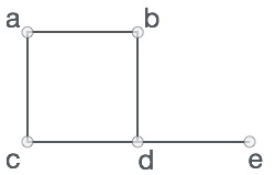
In the above graph,
V = {a, b, c, d, e}
E = {ab, ac, bd, cd, de}
Graph Data Structure
Mathematical graphs can be represented in data structure. We can represent a graph using an array of vertices and a two-dimensional array of edges. Before we proceed further, let's familiarize ourselves with some important terms −
Vertex − Each node of the graph is represented as a vertex. In the following example, the labeled circle represents vertices. Thus, A to G are vertices. We can represent them using an array as shown in the following image. Here A can be identified by index 0. B can be identified using index 1 and so on.
Edge − Edge represents a path between two vertices or a line between two vertices. In the following example, the lines from A to B, B to C, and so on represents edges. We can use a two-dimensional array to represent an array as shown in the following image. Here AB can be represented as 1 at row 0, column 1, BC as 1 at row 1, column 2 and so on, keeping other combinations as 0.
Adjacency − Two node or vertices are adjacent if they are connected to each other through an edge. In the following example, B is adjacent to A, C is adjacent to B, and so on.
Path − Path represents a sequence of edges between the two vertices. In the following example, ABCD represents a path from A to D.
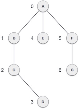
Basic Operations
Following are basic primary operations of a Graph −
Add Vertex − Adds a vertex to the graph.
Add Edge − Adds an edge between the two vertices of the graph.
Display Vertex − Displays a vertex of the graph.
To know more about Graph, please read Graph Theory Tutorial. We shall learn about traversing a graph in the coming chapters.
Data Structure - Depth First Traversal
Depth First Search (DFS) algorithm traverses a graph in a depthward motion and uses a stack to remember to get the next vertex to start a search, when a dead end occurs in any iteration.
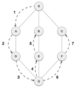
As in the example given above, DFS algorithm traverses from S to A to D to G to E to B first, then to F and lastly to C. It employs the following rules.
Rule 1 − Visit the adjacent unvisited vertex. Mark it as visited. Display it. Push it in a stack.
Rule 2 − If no adjacent vertex is found, pop up a vertex from the stack. (It will pop up all the vertices from the stack, which do not have adjacent vertices.)
Rule 3 − Repeat Rule 1 and Rule 2 until the stack is empty.
| Step | Traversal | Description |
|---|---|---|
| 1 | 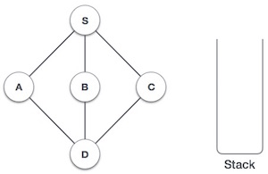 |
Initialize the stack. |
| 2 | 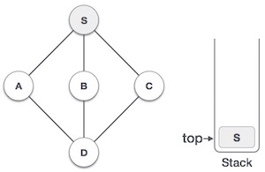 |
Mark S as visited and put it onto the stack. Explore any unvisited adjacent node from S. We have three nodes and we can pick any of them. For this example, we shall take the node in an alphabetical order. |
| 3 | 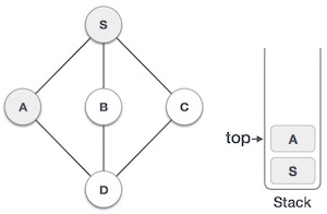 |
Mark A as visited and put it onto the stack. Explore any unvisited adjacent node from A. Both S and D are adjacent to A but we are concerned for unvisited nodes only. |
| 4 | 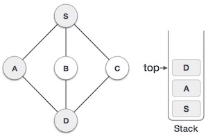 |
Visit D and mark it as visited and put onto the stack. Here, we have B and C nodes, which are adjacent to D and both are unvisited. However, we shall again choose in an alphabetical order. |
| 5 | 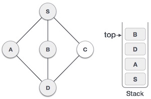 |
We choose B, mark it as visited and put onto the stack. Here B does not have any unvisited adjacent node. So, we pop B from the stack. |
| 6 | 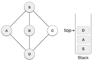 |
We check the stack top for return to the previous node and check if it has any unvisited nodes. Here, we find D to be on the top of the stack. |
| 7 | 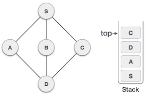 |
Only unvisited adjacent node is from D is C now. So we visit C, mark it as visited and put it onto the stack. |
As C does not have any unvisited adjacent node so we keep popping the stack until we find a node that has an unvisited adjacent node. In this case, there's none and we keep popping until the stack is empty.
To know about the implementation of this algorithm in C programming language, click here.
Data Structure - Breadth First Traversal
Breadth First Search (BFS) algorithm traverses a graph in a breadthward motion and uses a queue to remember to get the next vertex to start a search, when a dead end occurs in any iteration.

As in the example given above, BFS algorithm traverses from A to B to E to F first then to C and G lastly to D. It employs the following rules.
Rule 1 − Visit the adjacent unvisited vertex. Mark it as visited. Display it. Insert it in a queue.
Rule 2 − If no adjacent vertex is found, remove the first vertex from the queue.
Rule 3 − Repeat Rule 1 and Rule 2 until the queue is empty.
| Step | Traversal | Description |
|---|---|---|
| 1 | 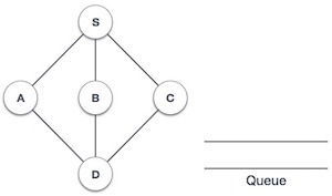 |
Initialize the queue. |
| 2 | 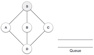 |
We start from visiting S (starting node), and mark it as visited. |
| 3 | 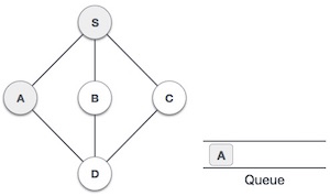 |
We then see an unvisited adjacent node from S. In this example, we have three nodes but alphabetically we choose A, mark it as visited and enqueue it. |
| 4 | 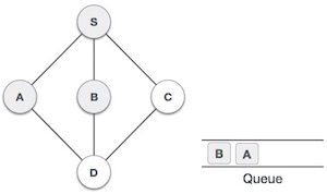 |
Next, the unvisited adjacent node from S is B. We mark it as visited and enqueue it. |
| 5 | 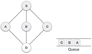 |
Next, the unvisited adjacent node from S is C. We mark it as visited and enqueue it. |
| 6 | 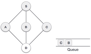 |
Now, S is left with no unvisited adjacent nodes. So, we dequeue and find A. |
| 7 | 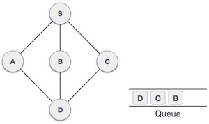 |
From A we have D as unvisited adjacent node. We mark it as visited and enqueue it. |
At this stage, we are left with no unmarked (unvisited) nodes. But as per the algorithm we keep on dequeuing in order to get all unvisited nodes. When the queue gets emptied, the program is over.
The implementation of this algorithm in C programming language can be seen here.
Data Structure and Algorithms - Tree
Tree represents the nodes connected by edges. We will discuss binary tree or binary search tree specifically.
Binary Tree is a special datastructure used for data storage purposes. A binary tree has a special condition that each node can have a maximum of two children. A binary tree has the benefits of both an ordered array and a linked list as search is as quick as in a sorted array and insertion or deletion operation are as fast as in linked list.
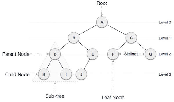
Important Terms
Following are the important terms with respect to tree.
Path − Path refers to the sequence of nodes along the edges of a tree.
Root − The node at the top of the tree is called root. There is only one root per tree and one path from the root node to any node.
Parent − Any node except the root node has one edge upward to a node called parent.
Child − The node below a given node connected by its edge downward is called its child node.
Leaf − The node which does not have any child node is called the leaf node.
Subtree − Subtree represents the descendants of a node.
Visiting − Visiting refers to checking the value of a node when control is on the node.
Traversing − Traversing means passing through nodes in a specific order.
Levels − Level of a node represents the generation of a node. If the root node is at level 0, then its next child node is at level 1, its grandchild is at level 2, and so on.
keys − Key represents a value of a node based on which a search operation is to be carried out for a node.
Binary Search Tree Representation
Binary Search tree exhibits a special behavior. A node's left child must have a value less than its parent's value and the node's right child must have a value greater than its parent value.
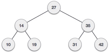
We're going to implement tree using node object and connecting them through references.
Tree Node
The code to write a tree node would be similar to what is given below. It has a data part and references to its left and right child nodes.
struct node {
   int data;
   struct node *leftChild;
   struct node *rightChild;
};
In a tree, all nodes share common construct.
BST Basic Operations
The basic operations that can be performed on a binary search tree data structure, are the following −
Insert − Inserts an element in a tree/create a tree.
Search − Searches an element in a tree.
Preorder Traversal − Traverses a tree in a pre-order manner.
Inorder Traversal − Traverses a tree in an in-order manner.
Postorder Traversal − Traverses a tree in a post-order manner.
We shall learn creating (inserting into) a tree structure and searching a data item in a tree in this chapter. We shall learn about tree traversing methods in the coming chapter.
Insert Operation
The very first insertion creates the tree. Afterwards, whenever an element is to be inserted, first locate its proper location. Start searching from the root node, then if the data is less than the key value, search for the empty location in the left subtree and insert the data. Otherwise, search for the empty location in the right subtree and insert the data.
Algorithm
If root is NULL
   then create root node
return

If root exists then
   compare the data with node.data

   while until insertion position is located

      If data is greater than node.data
         goto right subtree
      else
         goto left subtree

   endwhile

   insert data

end If
Implementation
The implementation of insert function should look like this −
void insert(int data) {
   struct node *tempNode = (struct node*) malloc(sizeof(struct node));
   struct node *current;
   struct node *parent;

   tempNode->data = data;
   tempNode->leftChild = NULL;
   tempNode->rightChild = NULL;

   //if tree is empty, create root node
   if(root == NULL) {
      root = tempNode;
   } else {
      current = root;
      parent  = NULL;

      while(1) {
         parent = current;

         //go to left of the tree
         if(data < parent->data) {
            current = current->leftChild;

            //insert to the left
            if(current == NULL) {
               parent->leftChild = tempNode;
               return;
            }
         }

         //go to right of the tree
         else {
            current = current->rightChild;

            //insert to the right
            if(current == NULL) {
               parent->rightChild = tempNode;
               return;
            }
         }
      }
   }
}
Search Operation
Whenever an element is to be searched, start searching from the root node, then if the data is less than the key value, search for the element in the left subtree. Otherwise, search for the element in the right subtree. Follow the same algorithm for each node.
Algorithm
If root.data is equal to search.data
   return root
else
   while data not found

      If data is greater than node.data
         goto right subtree
      else
         goto left subtree

      If data found
         return node
   endwhile

   return data not found

end if
The implementation of this algorithm should look like this.
struct node* search(int data) {
   struct node *current = root;
   printf("Visiting elements: ");

   while(current->data != data) {
      if(current != NULL)
      printf("%d ",current->data);

      //go to left tree

      if(current->data > data) {
         current = current->leftChild;
      }
      //else go to right tree
      else {
         current = current->rightChild;
      }

      //not found
      if(current == NULL) {
         return NULL;
      }

      return current;
   }
}
To know about the implementation of binary search tree data structure, please click here.
Data Structure & Algorithms - Tree Traversal
Traversal is a process to visit all the nodes of a tree and may print their values too. Because, all nodes are connected via edges (links) we always start from the root (head) node. That is, we cannot randomly access a node in a tree. There are three ways which we use to traverse a tree −
- In-order Traversal
- Pre-order Traversal
- Post-order Traversal
Generally, we traverse a tree to search or locate a given item or key in the tree or to print all the values it contains.
In-order Traversal
In this traversal method, the left subtree is visited first, then the root and later the right sub-tree. We should always remember that every node may represent a subtree itself.
If a binary tree is traversed in-order, the output will produce sorted key values in an ascending order.
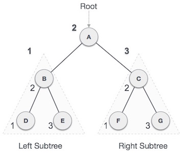
We start from A, and following in-order traversal, we move to its left subtree B. B is also traversed in-order. The process goes on until all the nodes are visited. The output of inorder traversal of this tree will be −
D → B → E → A → F → C → G
Algorithm
Until all nodes are traversed −
Step 1 − Recursively traverse left subtree.
Step 2 − Visit root node.
Step 3 − Recursively traverse right subtree.
Pre-order Traversal
In this traversal method, the root node is visited first, then the left subtree and finally the right subtree.
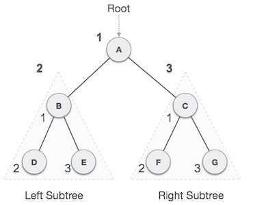
We start from A, and following pre-order traversal, we first visit A itself and then move to its left subtree B. B is also traversed pre-order. The process goes on until all the nodes are visited. The output of pre-order traversal of this tree will be −
A → B → D → E → C → F → G
Algorithm
Until all nodes are traversed −
Step 1 − Visit root node.
Step 2 − Recursively traverse left subtree.
Step 3 − Recursively traverse right subtree.
Post-order Traversal
In this traversal method, the root node is visited last, hence the name. First we traverse the left subtree, then the right subtree and finally the root node.
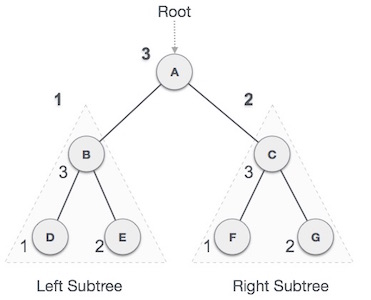
We start from A, and following Post-order traversal, we first visit the left subtree B. B is also traversed post-order. The process goes on until all the nodes are visited. The output of post-order traversal of this tree will be −
D → E → B → F → G → C → A
Algorithm
Until all nodes are traversed −
Step 1 − Recursively traverse left subtree.
Step 2 − Recursively traverse right subtree.
Step 3 − Visit root node.
To check the C implementation of tree traversing, please click here.
Data Structure - Binary Search Tree
A Binary Search Tree (BST) is a tree in which all the nodes follow the below-mentioned properties −
The left sub-tree of a node has a key less than or equal to its parent node's key.
The right sub-tree of a node has a key greater than to its parent node's key.
Thus, BST divides all its sub-trees into two segments; the left sub-tree and the right sub-tree and can be defined as −
left_subtree (keys) ≤ node (key) ≤ right_subtree (keys)
Representation
BST is a collection of nodes arranged in a way where they maintain BST properties. Each node has a key and an associated value. While searching, the desired key is compared to the keys in BST and if found, the associated value is retrieved.
Following is a pictorial representation of BST −
We observe that the root node key (27) has all less-valued keys on the left sub-tree and the higher valued keys on the right sub-tree.
Basic Operations
Following are the basic operations of a tree −
Search − Searches an element in a tree.
Insert − Inserts an element in a tree.
Pre-order Traversal − Traverses a tree in a pre-order manner.
In-order Traversal − Traverses a tree in an in-order manner.
Post-order Traversal − Traverses a tree in a post-order manner.
Node
Define a node having some data, references to its left and right child nodes.
struct node {
   int data;
   struct node *leftChild;
   struct node *rightChild;
};
Search Operation
Whenever an element is to be searched, start searching from the root node. Then if the data is less than the key value, search for the element in the left subtree. Otherwise, search for the element in the right subtree. Follow the same algorithm for each node.
Algorithm
struct node* search(int data){
   struct node *current = root;
   printf("Visiting elements: ");

   while(current->data != data){

      if(current != NULL) {
         printf("%d ",current->data);

         //go to left tree
         if(current->data > data){
            current = current->leftChild;
         }  //else go to right tree
         else {
            current = current->rightChild;
         }

         //not found
         if(current == NULL){
            return NULL;
         }
      }
   }

   return current;
}
Insert Operation
Whenever an element is to be inserted, first locate its proper location. Start searching from the root node, then if the data is less than the key value, search for the empty location in the left subtree and insert the data. Otherwise, search for the empty location in the right subtree and insert the data.
Algorithm
void insert(int data) {
   struct node *tempNode = (struct node*) malloc(sizeof(struct node));
   struct node *current;
   struct node *parent;

   tempNode->data = data;
   tempNode->leftChild = NULL;
   tempNode->rightChild = NULL;

   //if tree is empty
   if(root == NULL) {
      root = tempNode;
   } else {
      current = root;
      parent = NULL;

      while(1) {
         parent = current;

         //go to left of the tree
         if(data < parent->data) {
            current = current->leftChild;
            //insert to the left

            if(current == NULL) {
               parent->leftChild = tempNode;
               return;
            }
         }  //go to right of the tree
         else {
            current = current->rightChild;

            //insert to the right
            if(current == NULL) {
               parent->rightChild = tempNode;
               return;
            }
         }
      }
   }
}
Data Structure and Algorithms - AVL Trees
What if the input to binary search tree comes in a sorted (ascending or descending) manner? It will then look like this −
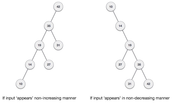
It is observed that BST's worst-case performance is closest to linear search algorithms, that is Ο(n). In real-time data, we cannot predict data pattern and their frequencies. So, a need arises to balance out the existing BST.
Named after their inventor Adelson, Velski & Landis, AVL trees are height balancing binary search tree. AVL tree checks the height of the left and the right sub-trees and assures that the difference is not more than 1. This difference is called the Balance Factor.
Here we see that the first tree is balanced and the next two trees are not balanced −
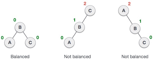
In the second tree, the left subtree of C has height 2 and the right subtree has height 0, so the difference is 2. In the third tree, the right subtree of A has height 2 and the left is missing, so it is 0, and the difference is 2 again. AVL tree permits difference (balance factor) to be only 1.
BalanceFactor = height(left-sutree) − height(right-sutree)
If the difference in the height of left and right sub-trees is more than 1, the tree is balanced using some rotation techniques.
AVL Rotations
To balance itself, an AVL tree may perform the following four kinds of rotations −
- Left rotation
- Right rotation
- Left-Right rotation
- Right-Left rotation
The first two rotations are single rotations and the next two rotations are double rotations. To have an unbalanced tree, we at least need a tree of height 2. With this simple tree, let's understand them one by one.
Left Rotation
If a tree becomes unbalanced, when a node is inserted into the right subtree of the right subtree, then we perform a single left rotation −
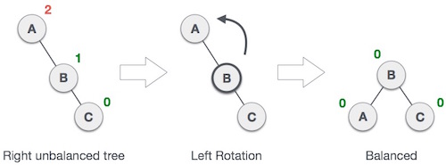
In our example, node A has become unbalanced as a node is inserted in the right subtree of A's right subtree. We perform the left rotation by making A the left-subtree of B.
Right Rotation
AVL tree may become unbalanced, if a node is inserted in the left subtree of the left subtree. The tree then needs a right rotation.
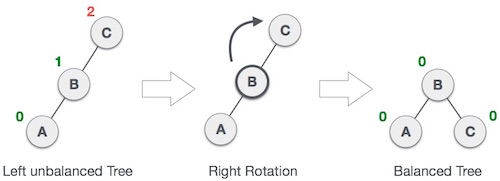
As depicted, the unbalanced node becomes the right child of its left child by performing a right rotation.
Left-Right Rotation
Double rotations are slightly complex version of already explained versions of rotations. To understand them better, we should take note of each action performed while rotation. Let's first check how to perform Left-Right rotation. A left-right rotation is a combination of left rotation followed by right rotation.
| State | Action |
|---|---|
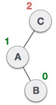 |
A node has been inserted into the right subtree of the left subtree. This makes C an unbalanced node. These scenarios cause AVL tree to perform left-right rotation. |
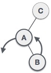 |
We first perform the left rotation on the left subtree of C. This makes A, the left subtree of B. |
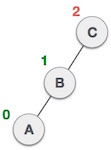 |
Node C is still unbalanced, however now, it is because of the left-subtree of the left-subtree. |
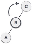 |
We shall now right-rotate the tree, making B the new root node of this subtree. C now becomes the right subtree of its own left subtree. |
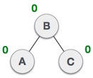 |
The tree is now balanced. |
Right-Left Rotation
The second type of double rotation is Right-Left Rotation. It is a combination of right rotation followed by left rotation.
| State | Action |
|---|---|
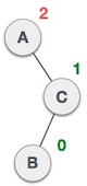 |
A node has been inserted into the left subtree of the right subtree. This makes A, an unbalanced node with balance factor 2. |
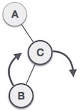 |
First, we perform the right rotation along C node, making C the right subtree of its own left subtree B. Now, B becomes the right subtree of A. |
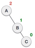 |
Node A is still unbalanced because of the right subtree of its right subtree and requires a left rotation. |
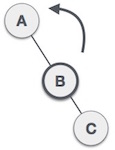 |
A left rotation is performed by making B the new root node of the subtree. A becomes the left subtree of its right subtree B. |
|
The tree is now balanced. |
Data Structure & Algorithms - Spanning Tree
A spanning tree is a subset of Graph G, which has all the vertices covered with minimum possible number of edges. Hence, a spanning tree does not have cycles and it cannot be disconnected..
By this definition, we can draw a conclusion that every connected and undirected Graph G has at least one spanning tree. A disconnected graph does not have any spanning tree, as it cannot be spanned to all its vertices.
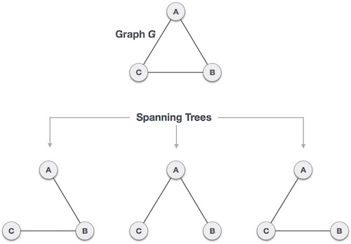
We found three spanning trees off one complete graph. A complete undirected graph can have maximum nn-2 number of spanning trees, where n is the number of nodes. In the above addressed example, n is 3, hence 33−2 = 3 spanning trees are possible.
General Properties of Spanning Tree
We now understand that one graph can have more than one spanning tree. Following are a few properties of the spanning tree connected to graph G −
A connected graph G can have more than one spanning tree.
All possible spanning trees of graph G, have the same number of edges and vertices.
The spanning tree does not have any cycle (loops).
Removing one edge from the spanning tree will make the graph disconnected, i.e. the spanning tree is minimally connected.
Adding one edge to the spanning tree will create a circuit or loop, i.e. the spanning tree is maximally acyclic.
Mathematical Properties of Spanning Tree
Spanning tree has n-1 edges, where n is the number of nodes (vertices).
From a complete graph, by removing maximum e - n + 1 edges, we can construct a spanning tree.
A complete graph can have maximum nn-2 number of spanning trees.
Thus, we can conclude that spanning trees are a subset of connected Graph G and disconnected graphs do not have spanning tree.
Application of Spanning Tree
Spanning tree is basically used to find a minimum path to connect all nodes in a graph. Common application of spanning trees are −
Civil Network Planning
Computer Network Routing Protocol
Cluster Analysis
Let us understand this through a small example. Consider, city network as a huge graph and now plans to deploy telephone lines in such a way that in minimum lines we can connect to all city nodes. This is where the spanning tree comes into picture.
Minimum Spanning Tree (MST)
In a weighted graph, a minimum spanning tree is a spanning tree that has minimum weight than all other spanning trees of the same graph. In real-world situations, this weight can be measured as distance, congestion, traffic load or any arbitrary value denoted to the edges.
Minimum Spanning-Tree Algorithm
We shall learn about two most important spanning tree algorithms here −
Both are greedy algorithms.
Heap Data Structures
Heap is a special case of balanced binary tree data structure where the root-node key is compared with its children and arranged accordingly. If α has child node β then −
key(α) ≥ key(β)
As the value of parent is greater than that of child, this property generates Max Heap. Based on this criteria, a heap can be of two types −
For Input → 35 33 42 10 14 19 27 44 26 31
Min-Heap − Where the value of the root node is less than or equal to either of its children.
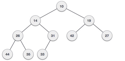
Max-Heap − Where the value of the root node is greater than or equal to either of its children.
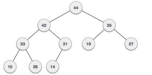
Both trees are constructed using the same input and order of arrival.
Max Heap Construction Algorithm
We shall use the same example to demonstrate how a Max Heap is created. The procedure to create Min Heap is similar but we go for min values instead of max values.
We are going to derive an algorithm for max heap by inserting one element at a time. At any point of time, heap must maintain its property. While insertion, we also assume that we are inserting a node in an already heapified tree.
Step 1 − Create a new node at the end of heap.
Step 2 − Assign new value to the node.
Step 3 − Compare the value of this child node with its parent.
Step 4 − If value of parent is less than child, then swap them.
Step 5 − Repeat step 3 & 4 until Heap property holds.
Note − In Min Heap construction algorithm, we expect the value of the parent node to be less than that of the child node.
Let's understand Max Heap construction by an animated illustration. We consider the same input sample that we used earlier.
Max Heap Deletion Algorithm
Let us derive an algorithm to delete from max heap. Deletion in Max (or Min) Heap always happens at the root to remove the Maximum (or minimum) value.
Step 1 − Remove root node.
Step 2 − Move the last element of last level to root.
Step 3 − Compare the value of this child node with its parent.
Step 4 − If value of parent is less than child, then swap them.
Step 5 − Repeat step 3 & 4 until Heap property holds.
Data Structure - Recursion Basics
Some computer programming languages allow a module or function to call itself. This technique is known as recursion. In recursion, a function α either calls itself directly or calls a function β that in turn calls the original function α. The function α is called recursive function.
Example − a function calling itself.
int function(int value) {
   if(value < 1)
      return;
   function(value - 1);

   printf("%d ",value);
}
Example − a function that calls another function which in turn calls it again.
int function1(int value1) {
   if(value1 < 1)
      return;
   function2(value1 - 1);
   printf("%d ",value1);
}
int function2(int value2) {
   function1(value2);
}
Properties
A recursive function can go infinite like a loop. To avoid infinite running of recursive function, there are two properties that a recursive function must have −
Base criteria − There must be at least one base criteria or condition, such that, when this condition is met the function stops calling itself recursively.
Progressive approach − The recursive calls should progress in such a way that each time a recursive call is made it comes closer to the base criteria.
Implementation
Many programming languages implement recursion by means of stacks. Generally, whenever a function (caller) calls another function (callee) or itself as callee, the caller function transfers execution control to the callee. This transfer process may also involve some data to be passed from the caller to the callee.
This implies, the caller function has to suspend its execution temporarily and resume later when the execution control returns from the callee function. Here, the caller function needs to start exactly from the point of execution where it puts itself on hold. It also needs the exact same data values it was working on. For this purpose, an activation record (or stack frame) is created for the caller function.

This activation record keeps the information about local variables, formal parameters, return address and all information passed to the caller function.
Analysis of Recursion
One may argue why to use recursion, as the same task can be done with iteration. The first reason is, recursion makes a program more readable and because of latest enhanced CPU systems, recursion is more efficient than iterations.
Time Complexity
In case of iterations, we take number of iterations to count the time complexity. Likewise, in case of recursion, assuming everything is constant, we try to figure out the number of times a recursive call is being made. A call made to a function is Ο(1), hence the (n) number of times a recursive call is made makes the recursive function Ο(n).
Space Complexity
Space complexity is counted as what amount of extra space is required for a module to execute. In case of iterations, the compiler hardly requires any extra space. The compiler keeps updating the values of variables used in the iterations. But in case of recursion, the system needs to store activation record each time a recursive call is made. Hence, it is considered that space complexity of recursive function may go higher than that of a function with iteration.
Data Structure & Algorithms - Tower of Hanoi
Tower of Hanoi, is a mathematical puzzle which consists of three towers (pegs) and more than one rings is as depicted −
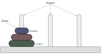
These rings are of different sizes and stacked upon in an ascending order, i.e. the smaller one sits over the larger one. There are other variations of the puzzle where the number of disks increase, but the tower count remains the same.
Rules
The mission is to move all the disks to some another tower without violating the sequence of arrangement. A few rules to be followed for Tower of Hanoi are −
- Only one disk can be moved among the towers at any given time.
- Only the "top" disk can be removed.
- No large disk can sit over a small disk.
Following is an animated representation of solving a Tower of Hanoi puzzle with three disks.
Tower of Hanoi puzzle with n disks can be solved in minimum 2n−1 steps. This presentation shows that a puzzle with 3 disks has taken 23 - 1 = 7 steps.
Algorithm
To write an algorithm for Tower of Hanoi, first we need to learn how to solve this problem with lesser amount of disks, say → 1 or 2. We mark three towers with name, source, destination and aux (only to help moving the disks). If we have only one disk, then it can easily be moved from source to destination peg.
If we have 2 disks −
- First, we move the smaller (top) disk to aux peg.
- Then, we move the larger (bottom) disk to destination peg.
- And finally, we move the smaller disk from aux to destination peg.
So now, we are in a position to design an algorithm for Tower of Hanoi with more than two disks. We divide the stack of disks in two parts. The largest disk (nth disk) is in one part and all other (n-1) disks are in the second part.
Our ultimate aim is to move disk n from source to destination and then put all other (n1) disks onto it. We can imagine to apply the same in a recursive way for all given set of disks.
The steps to follow are −
Step 1 − Move n-1 disks fromsourcetoauxStep 2 − Move nth disk fromsourcetodestStep 3 − Move n-1 disks fromauxtodest
A recursive algorithm for Tower of Hanoi can be driven as follows −
START
Procedure Hanoi(disk, source, dest, aux)

   IF disk == 1, THEN
      move disk from source to dest
   ELSE
      Hanoi(disk - 1, source, aux, dest)     // Step 1
      move disk from source to dest          // Step 2
      Hanoi(disk - 1, aux, dest, source)     // Step 3
   END IF

END Procedure
STOP
To check the implementation in C programming, click here.
Data Structure & Algorithms Fibonacci Series
Fibonacci series generates the subsequent number by adding two previous numbers. Fibonacci series starts from two numbers − F0 & F1. The initial values of F0 & F1 can be taken 0, 1 or 1, 1 respectively.
Fibonacci series satisfies the following conditions −
Fn = Fn-1 + Fn-2
Hence, a Fibonacci series can look like this −
F8 = 0 1 1 2 3 5 8 13
or, this −
F8 = 1 1 2 3 5 8 13 21
For illustration purpose, Fibonacci of F8 is displayed as −
Fibonacci Iterative Algorithm
First we try to draft the iterative algorithm for Fibonacci series.
Procedure Fibonacci(n)
   declare f0, f1, fib, loop

   set f0 to 0
   set f1 to 1

   display f0, f1

   for loop ← 1 to n

      fib ← f0 + f1
      f0 ← f1
      f1 ← fib

      display fib
   end for

end procedure
To know about the implementation of the above algorithm in C programming language, click here.
Fibonacci Recursive Algorithm
Let us learn how to create a recursive algorithm Fibonacci series. The base criteria of recursion.
START
Procedure Fibonacci(n)
   declare f0, f1, fib, loop

   set f0 to 0
   set f1 to 1

   display f0, f1

   for loop ← 1 to n

      fib ← f0 + f1
      f0 ← f1
      f1 ← fib

      display fib
   end for

END
To see the implementation of above algorithm in c programming language, click here.


