Pandas is one of the most popular python library for data science and analytics. Pandas library is used for data manipulation, analysis and cleaning. It is a high-level abstraction over low-level NumPy which is written purely in C. In this section, we will cover some of the most important (most often used) things we need to know as an anayst or a data scientist.
We can install the required libraries using pip, simply run below command on your command terminal:
pip intall pandas
First we need to understand two main basic data structure of pandas .i.e. DataFrame and Series. We need to have solid understanding of these two data structure in order to master pandas.
Series is an object which is similar to python built-in type list but differs from it because it has associated lable with each element or index.
>>> import pandas as pd
>>> my_series = pd.Series([12, 24, 36, 48, 60, 72, 84])
>>> my_series
0 12
1 24
2 36
3 48
4 60
5 72
6 84
dtype: int64
In the above output, the ‘index’ is on the left side and ‘value’ on the right. Also each Series object has data type(dtype), in our case its int64.
We can retrieve elements by their index number:
>>> my_series[6]
84
To provide index(labels) explicity, use:
>>> my_series = pd.Series([12, 24, 36, 48, 60, 72, 84], index =['ind0', 'ind1', 'ind2', 'ind3', 'ind4', 'ind5', 'ind6'])
>>> my_series
ind0 12
ind1 24
ind2 36
ind3 48
ind4 60
ind5 72
ind6 84
dtype: int64
Also it is very easy to retrieve several elements by their indexes or make group assignment:
>>> my_series[['ind0', 'ind3', 'ind6']]
ind0 12
ind3 48
ind6 84
dtype: int64
>>> my_series[['ind0', 'ind3', 'ind6']] = 36
>>> my_series
ind0 36
ind1 24
ind2 36
ind3 36
ind4 60
ind5 72
ind6 36
dtype: int64
Filtering and math operations are easy as well:
>>> my_series[my_series>24]
ind0 36
ind2 36
ind3 36
ind4 60
ind5 72
ind6 36
dtype: int64
>>> my_series[my_series < 24] * 2
Series([], dtype: int64)
>>> my_series
ind0 36
ind1 24
ind2 36
ind3 36
ind4 60
ind5 72
ind6 36
dtype: int64
>>>
Below are some other common operations on Series.
>>> #Work as dictionaries
>>> my_series1 = pd.Series({'a':9, 'b':18, 'c':27, 'd': 36})
>>> my_series1
a 9
b 18
c 27
d 36
dtype: int64
>>> #Label attributes
>>> my_series1.name = 'Numbers'
>>> my_series1.index.name = 'letters'
>>> my_series1
letters
a 9
b 18
c 27
d 36
Name: Numbers, dtype: int64
>>> #chaning Index
>>> my_series1.index = ['w', 'x', 'y', 'z']
>>> my_series1
w 9
x 18
y 27
z 36
Name: Numbers, dtype: int64
>>>
DataFrame acts like a table as it contains rows and columns. Each column in a DataFrame is a Series object and rows consist of elements inside Series.
DataFrame can be constructed using built-in Python dicts:
>>> df = pd.DataFrame({
   'Country': ['China', 'India', 'Indonesia', 'Pakistan'],
   'Population': [1420062022, 1368737513, 269536482, 204596442],
   'Area' : [9388211, 2973190, 1811570, 770880]
})
>>> df
  Area     Country    Population
0 9388211  China      1420062022
1 2973190  India      1368737513
2 1811570  Indonesia  269536482
3 770880   Pakistan   204596442
>>> df['Country']
0 China
1 India
2 Indonesia
3 Pakistan
Name: Country, dtype: object
>>> df.columns
Index(['Area', 'Country', 'Population'], dtype='object')
>>> df.index
RangeIndex(start=0, stop=4, step=1)
>>>There are several ways to provide row index explicitly.
>>> df = pd.DataFrame({
   'Country': ['China', 'India', 'Indonesia', 'Pakistan'],
   'Population': [1420062022, 1368737513, 269536482, 204596442],
   'Landarea' : [9388211, 2973190, 1811570, 770880]
}, index = ['CHA', 'IND', 'IDO', 'PAK'])
>>> df
Country Landarea Population
CHA China 9388211 1420062022
IND India 2973190 1368737513
IDO Indonesia 1811570 269536482
PAK Pakistan 770880 204596442
>>> df.index = ['CHI', 'IND', 'IDO', 'PAK']
>>> df.index.name = 'Country Code'
>>> df
Country Landarea Population
Country Code
CHI China 9388211 1420062022
IND India 2973190 1368737513
IDO Indonesia 1811570 269536482
PAK Pakistan 770880 204596442
>>> df['Country']
Country Code
CHI China
IND India
IDO Indonesia
PAK Pakistan
Name: Country, dtype: object
Row access using index can be performed in several ways
>>> df.loc['IND']
Country         India
Landarea      2973190
Population 1368737513
Name: IND, dtype: object
>>> df.iloc[1]
Country         India
Landarea      2973190
Population 1368737513
Name: IND, dtype: object
>>>
>>> df.loc[['CHI', 'IND'], 'Population']
Country Code
CHI      1420062022
IND      1368737513
Name: Population, dtype: int64
Pandas supports many popular file formats including CSV, XML, HTML, Excel, SQL, JSON many more. Most commonly CSV file format is used.
To read a csv file, just run:
>>> df = pd.read_csv('GDP.csv', sep = ',')Named argument sep points to a separator character in CSV file called GDP.csv.
In order to group data in pandas we can use .groupby method. To demonstrate the use of aggregates and grouping in pandas I have used the Titanic dataset, you can find the same from below link:
https://yadi.sk/d/TfhJdE2k3EyALt
>>> titanic_df = pd.read_csv('titanic.csv')
>>> print(titanic_df.head())
PassengerID                                   Name  PClass
Age \
0                        1 Allen, Miss Elisabeth Walton 1st
29.00
1 2                         Allison, Miss Helen Loraine 1st
2.00
2 3                 Allison, Mr Hudson Joshua Creighton 1st
30.00
3 4       Allison, Mrs Hudson JC (Bessie Waldo Daniels) 1st
25.00
4 5                  Allison, Master Hudson Trevor 1st 0.92

     Sex      Survived      SexCode
0  female        1             1
1  female        0             1
2  male          0             0
3  female        0             1
4  male          1             0
>>>
Let’s calculate how many passengers (women and men) survived and how many did not, we will use .groupby
>>> print(titanic_df.groupby(['Sex', 'Survived'])['PassengerID'].count())
Sex         Survived
female       0          154
             1          308
male         0          709
             1          142
Name: PassengerID, dtype: int64
Above data based on cabin class:
>>> print(titanic_df.groupby(['PClass', 'Survived'])['PassengerID'].count())
PClass    Survived
*         0              1
1st       0              129
          1              193
2nd       0              160
          1              119
3rd       0              573
          1              138
Name: PassengerID, dtype: int64
Pandas was created to analyse time series data. In order to illustrate, I have used the amazon 5 years stock prices. You can download it from below link,
>>> import pandas as pd
>>> amzn_df = pd.read_csv('AMZN.csv', index_col='Date', parse_dates=True)
>>> amzn_df = amzn_df.sort_index()
>>> print(amzn_df.info())
<class 'pandas.core.frame.DataFrame'>
DatetimeIndex: 62 entries, 2014-04-01 to 2019-04-12
Data columns (total 6 columns):
Open         62 non-null object
High         62 non-null object
Low          62 non-null object
Close        62 non-null object
Adj Close    62 non-null object
Volume       62 non-null object
dtypes: object(6)
memory usage: 1.9+ KB
None
Above we have created a DataFRame with DatetimeIndex by Date column and then sort it.
And the mean closing price is,
>>> amzn_df.loc['2015-04', 'Close'].mean()
421.779999
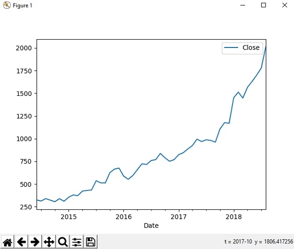
We can use matplotlib library to visualize pandas. Let’s take our amazon stock historical dataset and look into its price movement of specific time period over graph.
>>> import matplotlib.pyplot as plt
>>> df = pd.read_csv('AMZN.csv', index_col = 'Date' , parse_dates = True)
>>> new_df = df.loc['2014-06':'2018-08', ['Close']]
>>> new_df=new_df.astype(float)
>>> new_df.plot()
<matplotlib.axes._subplots.AxesSubplot object at 0x0B9B8930>
>>> plt.show()