SAS - Bland Altman Analysis
The Bland-Altman analysis is a process to verify the extent of agreement or disagreement between two methods designed to measure same parameters. A high correlation between the methods indicate that good enough sample has been chosen in data analysis. In SAS we create a Bland-Altman plot by calculating the mean, upper limit and lower limit of the variable values. We then use PROC SGPLOT to create the Bland-Altman plot.
Syntax
The basic syntax for applying PROC SGPLOT in SAS is −
PROC SGPLOT DATA = dataset;
SCATTER X = variable Y = Variable;
REFLINE value;
Following is the description of the parameters used −
Dataset is the name of the dataset.
SCATTER statement cerates the scatter plot graph of the value supplied in form of X and Y.
REFLINE creates a horizontal or vertical reference line.
Example
In the below example we take the result of two experiments generated by two methods named new and old. We calculate the differences in the values of the variables and also the mean of the variables of the same observation. We also calculate the standard deviation values to be used in the upper and lower limit of the calculation.
The result shows a Bland-Altman plot as a scatter plot.
data mydata;
input new old;
datalines;
31 45
27 12
11 37
36 25
14 8
27 15
3 11
62 42
38 35
20 9
35 54
62 67
48 25
77 64
45 53
32 42
16 19
15 27
22 9
8 38
24 16
59 25
;
data diffs ;
set mydata ;
/* calculate the difference */
diff = new-old ;
/* calculate the average */
mean = (new+old)/2 ;
run ;
proc print data = diffs;
run;
proc sql noprint ;
select mean(diff)-2*std(diff), mean(diff)+2*std(diff)
into :lower, :upper
from diffs ;
quit;
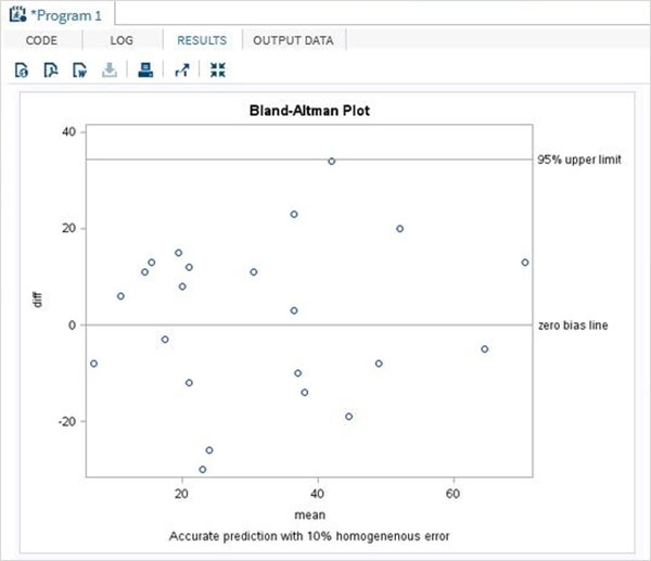
proc sgplot data = diffs ;
scatter x = mean y = diff;
refline 0 &upper &lower / LABEL = ("zero bias line" "95% upper limit" "95%
lower limit");
TITLE 'Bland-Altman Plot';
footnote 'Accurate prediction with 10% homogeneous error';
run ;
quit ;
When the above code is executed, we get the following result −
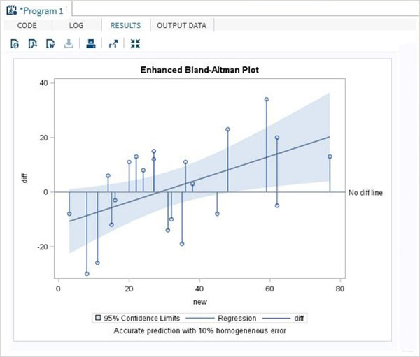
Enhanced Model
In an enhanced model of the above program we get 95 percent confidence level curve fitting.
proc sgplot data = diffs ;
reg x = new y = diff/clm clmtransparency = .5;
needle x = new y = diff/baseline = 0;
refline 0 / LABEL = ('No diff line');
TITLE 'Enhanced Bland-Altman Plot';
footnote 'Accurate prediction with 10% homogeneous error';
run ;
quit ;
When the above code is executed, we get the following result −