SAS - Quick Guide

SAS - Overview

SAS stands for Statistical Analysis Software. It was created in the year 1960 by the SAS Institute. From 1st January 1960, SAS was used for data management, business intelligence, Predictive Analysis, Descriptive and Prescriptive Analysis etc. Since then, many new statistical procedures and components were introduced in the software.

With the introduction of JMP (Jump) for statistics SAS took advantage of the Graphical user Interface which was introduced by the Macintosh. Jump is basically used for the applications like Six Sigma, designs, quality control and engineering and scientific analysis.

SAS is platform independent which means you can run SAS on any operating system either Linux or Windows. SAS is driven by SAS programmers who use several sequences of operations on the SAS datasets to make proper reports for data analysis.

Over the years SAS has added numerous solutions to its product portfolio. It has solution for Data Governance, Data Quality, Big Data Analytics, Text Mining, Fraud management, Health science etc. We can safely assume SAS has a solution for every business domain.

To have a glance at the list of products available you can visit SAS Components

Why we use SAS

SAS is basically worked on large datasets. With the help of SAS software you can perform various operations on the data like −

Data Management
Statistical Analysis
Report formation with perfect graphics
Business Planning
Operations Research and project Management
Quality Improvement
Application Development
Data extraction
Data transformation
Data updation and modification

If we talk about the components of SAS then more than 200 components are available in SAS.

Sr.No.	SAS Component & their Usage
1	Base SAS It is a core component which contains data management facility and a programming language for data analysis. It is also the most widely used.
2	SAS/GRAPH Create graphs, presentations for better understanding and showcasing the result in a proper format.
3	SAS/STAT Perform Statistical analysis with the variance analysis, regression, multivariate analysis, survival analysis, and psychometric analysis, mixed model analysis.
4	SAS/OR Operations research.
5	SAS/ETS Econometrics and Time Series Analysis.
6	SAS/IML CInteractive matrix language.
7	SAS/AF Applications facility.
8	SAS/QC Quality control.
9	SAS/INSIGHT Data mining.
10	SAS/PH Clinical trial analysis.
11	SAS/Enterprise Miner Data mining.

Types of SAS Software

Windows or PC SAS
SAS EG (Enterprise Guide)
SAS EM (Enterprise Miner i.e. for Predictive Analysis)
SAS Means
SAS Stats

Mostly we use Window SAS in organisation as well as in training institute. Some of the organisations use Linux but there is no graphical user interface so you have to write code for every query. But in window SAS there are a lot of utilities available which helps the programmers very much and it also reduces the time of writing the codes as well.

A SaS Window have 5 parts.

Sr.No.	SAS Window & their Usage
1	Log Window A log window is like an execution window where we can check the execution of the SAS program. In this window we can check the errors also. It is very important to check every time the log window after running the program. So that we can have proper understanding about the execution of our program.
2	Editor Window Editor Window is that part of SAS where we write all the codes. It is like a notepad.
3	Output Window Output window is the result window where we can see the output of our program.
4	Result Window It is like an index to all the outputs. All the programs that we have run in one session of the SAS are listed there and you can open the output by clicking on the output result. But these are mentioned only in one session of the SAS. If we close the software and then open it then the Result Window will be empty.
5	Explore Window Here all the libraries listed. You can also browse your system SAS supported files from here.

Libraries in SAS

Libraries are like storage in SAS. You can create a library and save all the similar programs in that library. SAS provides you the facility to create multiple libraries. A SAS library is only 8 characters long.

There are two types of libraries are available in SAS −

Sr.No.	SAS Window & their Usage
1	Temporary or Work Library This is the by default library of SAS. All the programs that we create are stored in this work library if we do not assign any other library to them. You can check this work library in the Explore Window. If you create a SAS program and have not assign any permanent library to it then if you end the session after that again you start the software then this program will not be in the work library. Because it will only be there in Work library as long as the session goes ones.
2	Permanent Library These are the permanent libraries of SAS. We can create a new SAS library by using SAS utilities or by writing the codes in the editor window. These libraries are named as permanent because if we create a program in SAS and save it in these permanent libraries then these will be available as long as we want them.

Sr.No.

SAS Window & their Usage

Temporary or Work Library

This is the by default library of SAS. All the programs that we create are stored in this work library if we do not assign any other library to them. You can check this work library in the Explore Window. If you create a SAS program and have not assign any permanent library to it then if you end the session after that again you start the software then this program will not be in the work library. Because it will only be there in Work library as long as the session goes ones.

Permanent Library

These are the permanent libraries of SAS. We can create a new SAS library by using SAS utilities or by writing the codes in the editor window. These libraries are named as permanent because if we create a program in SAS and save it in these permanent libraries then these will be available as long as we want them.

SAS - Environment

SAS Institute Inc. has released a free SAS University Edition which is good enough for learning SAS programming. It provides all the features that you need to learn in BASE SAS programming which in turn enables you to learn any other SAS component.

The process of downloading and installing SAS University Edition is very straight forward. It is available as a virtual machine which needs to run on a virtual environment. You need to have virtualization software already installed in your PC before you can run the SAS software. In this tutorial we will be using VMware. Below are the details of the steps to download, setup the SAS environment and verify the installation.

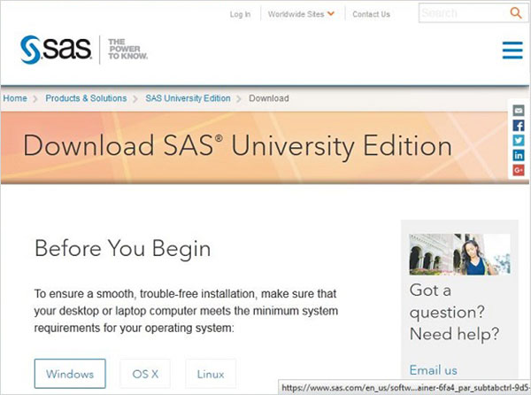
Download SAS University Edition

SAS University Edition is available for download at the URL SAS University Edition. Please scroll down to read the system requirements before you begin the download. The following screen appears on visiting this URL.

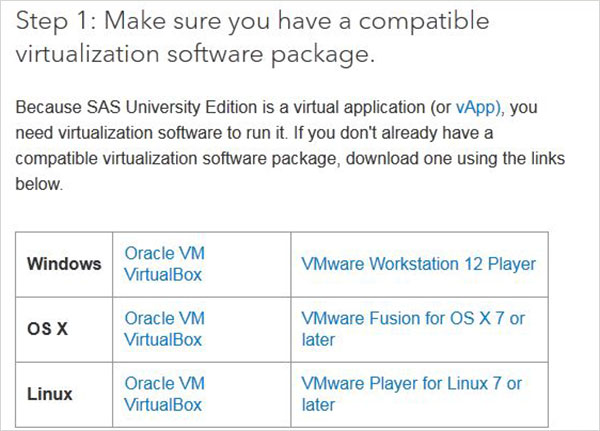
Setup virtualization software

Scroll down on the same page to locate the installation stpe-1. This step provides the links to get the virtualization software that suits you. In case you already have any one of these softwares installed in your system, you can skip this step.

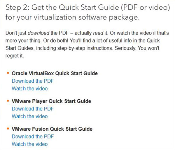
Quick start virtualization software

In case you are completely new to virtualization environment, you can familiarize yourself with it by going through the following guides and videos available as step-2. Again you can skip this step in case you are already familiar.

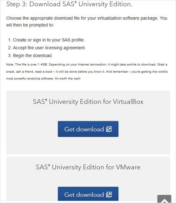
Download the Zip file

In step-3 you can choose the appropriate version of the SAS University Edition compatible with the virtualization environment you have. It downloads as a zip file with name similar to unvbasicvapp__9411005__vmx__en__sp0__1.zip

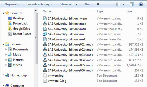
Unzip the zip file

The zip file above needs to be unzipped and stored in an appropriate directory. In our case we have chosen the VMware zip file which shows the following files after unzipping.

Loading the virtual machine

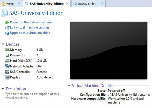
Start the VMware player (or workstation) and open the file which ends with an extension .vmx. The below screen appears. Please notice the basic settings like memory and hard disk space allocated to the vm.

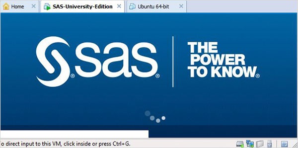
Power on the virtual machine

Click the Power on this virtual machine alongside the green arrow mark to start the virtual machine. The following screen appears.

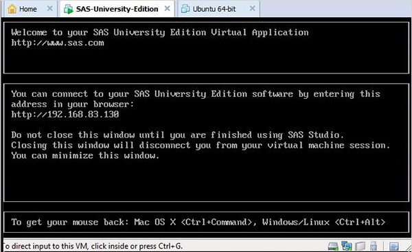
The below screen appears when the SAS vm is in the state of loading after which the running vm gives a prompt to go to a URL location which will open the SAS environment.

Starting SAS studio

Open a new browser tab and load the above URL (which differs from one PC to another). The below screen appears indicating the SAS environment is ready.

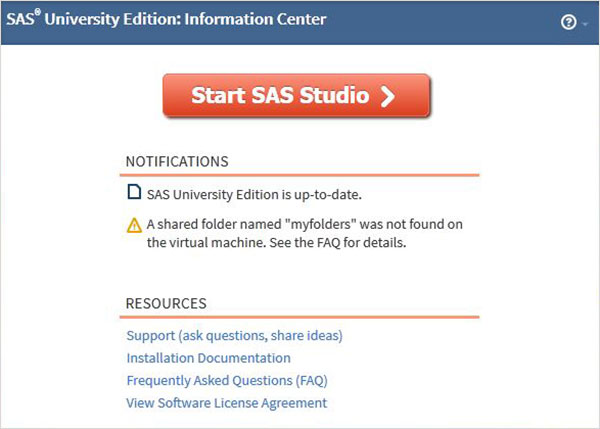
The SAS Environment

On clicking the Start SAS Studio we get the SAS environment which by default opens in the visual programmer mode as shown below.

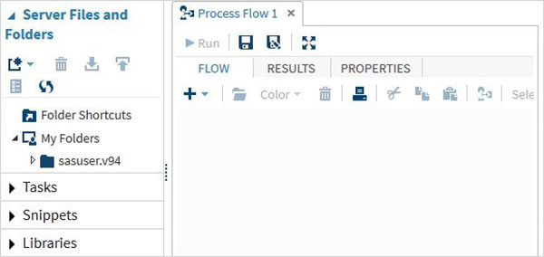
We can also change it to SAS programmer mode by clicking on the drop down.

Now we are ready to write SAS Programs.

SAS - User Interface

SAS Programs are created using a user interface known as SAS Studio.

Below is a description of various windows and their usage.

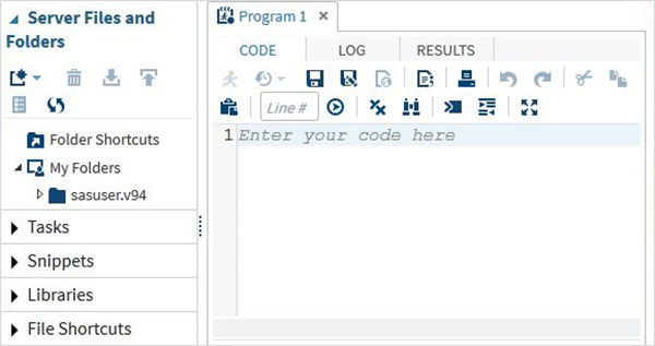
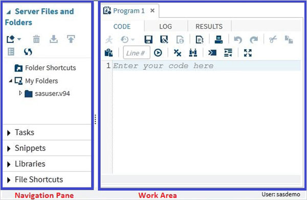
SAS Main Window

This is the window you see on entering the SAS environment. In the left is the Navigation Paneused to navigate various programming features. In the right is the Work Area which is used for writing the code and executing it.

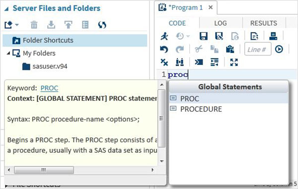
Code Autocomplete

This is a very powerful feature which helps getting the correct syntax of SAS keywords as well as provides link to the documentation for that keyword.

Program Execution

The execution of code is done by pressing the run icon, which is the first icon from left or the F3 button.

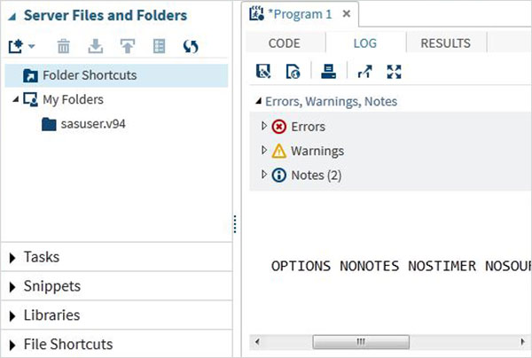
Program Log

The log of the executed code is available under the Log tab. It describes the errors, warnings or notes about the program’s execution. This is the window where you get all the clues to troubleshoot your code.

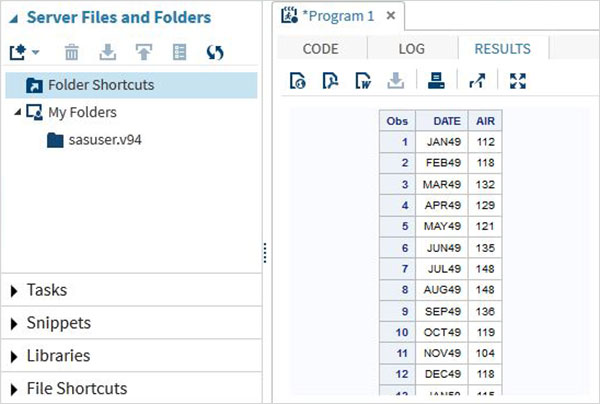
Program Result

The result of the code execution is seen in the RESULTS tab. By default they are formatted as html tables.

Program Tabs

The Navigation Area contains features to create and manage programs. It also provides the pre-built functionalities to be used with your program.

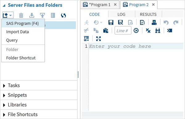
Server Files and Folders

Under this tab we can create additional programs, import data to be analyzed and query the existing data. It can also be used to create folder shortcuts.

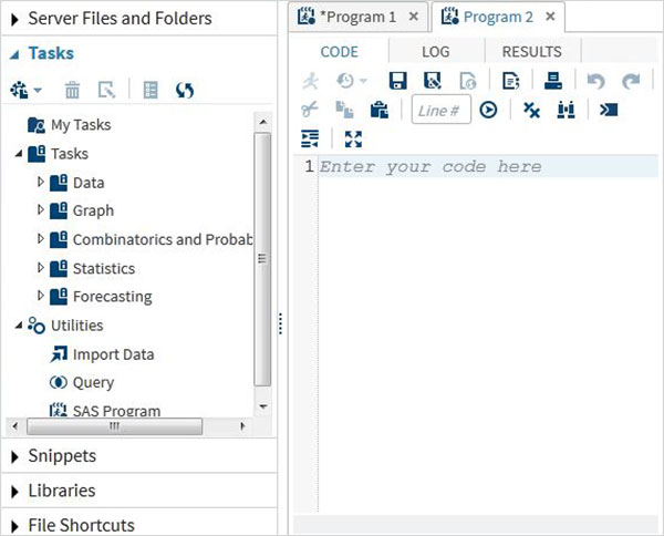
Tasks

The Tasks tab provides features to use in-built SAS programs by supplying only the input variables. For example under the statistics folder you can find a SAS program to do linear regression by only supplying the SAS data set name and variable names.

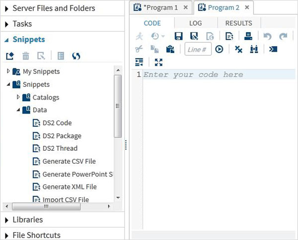
Snippets

The snippets tab provides features to write SAS Macro and generate files from the existing data set

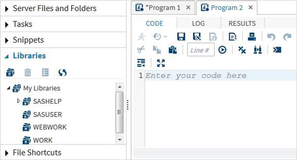
Program Libraries

SAS stores the datasets in SAS libraries. The temporary library is available only for a single session and it is named as WORK. But the permanent libraries are available always.

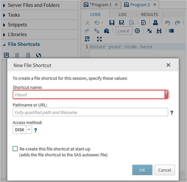
File Shortcuts

This tab is used to access files which are stored outside the SAS environment. The shortcuts to such files are stored under this tab.

SAS - Program Structure

The SAS Programming involves first creating/reading the data sets into the memory and then doing the analysis on this data. We need to understand the flow in which a program is written to achieve this.

SAS Program Structure

The below diagram shows the steps to be written in the given sequence to create a SAS Program.

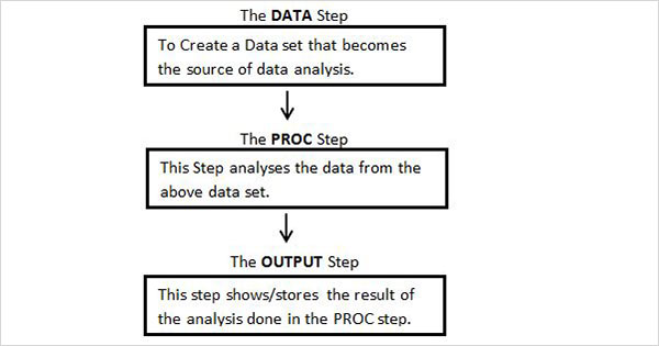
Every SAS program must have all these steps to complete reading the input data, analysing the data and giving the output of the analysis. Also the RUN statement at the end of each step is required to complete the execution of that step.

DATA Step

This step involves loading the required data set into SAS memory and identifying the variables (also called columns) of the data set. It also captures the records (also called observations or subjects). The syntax for DATA statement is as below.

Syntax

DATA data_set_name;		#Name the data set.
INPUT var1,var2,var3; 		#Define the variables in this data set.
NEW_VAR;			#Create new variables.
LABEL;			      	#Assign labels to variables.
DATALINES;		      	#Enter the data.
RUN;

Example

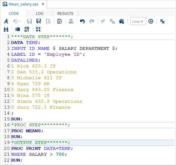
The below example shows a simple case of naming the data set, defining the variables, creating new variables and entering the data. Here the string variables have a $ at the end and numeric values are without it.

DATA TEMP;
INPUT ID $ NAME $ SALARY DEPARTMENT $;
comm = SALARY*0.25;
LABEL ID = 'Employee ID' comm = 'COMMISION';
DATALINES;
1 Rick 623.3 IT
2 Dan 515.2 Operations
3 Michelle 611 IT
4 Ryan 729 HR
5 Gary 843.25 Finance
6 Nina 578 IT
7 Simon 632.8 Operations
8 Guru 722.5 Finance
;
RUN;

PROC Step

This step involves invoking a SAS built-in procedure to analyse the data.

Syntax

PROC procedure_name options; #The name of the proc.
RUN;

Example

The below example shows using the MEANS procedure to print the mean values of the numeric variables in the data set.

PROC MEANS;
RUN;

The OUTPUT Step

The data from the data sets can be displayed with conditional output statements.

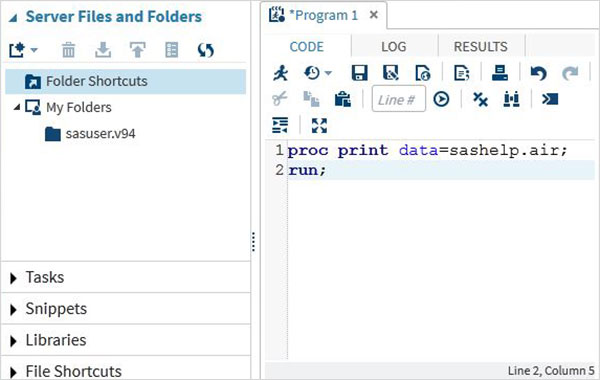
Syntax

PROC PRINT DATA = data_set;
OPTIONS;
RUN;

Example

The below example shows using the where clause in the output to produce only few records from the data set.

PROC PRINT DATA = TEMP;
WHERE SALARY > 700;
RUN;

The complete SAS Program

Below is the complete code for each of the above steps.

Program Output

The output from above code is seen in the RESULTS tab.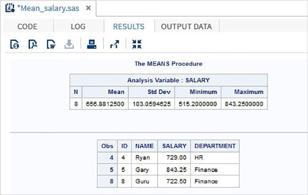

SAS - Basic Syntax

Like any other programming language, the SAS language has its own rules of syntax to create the SAS programs.

The three components of any SAS program - Statements, Variables and Data sets follow the below rules on Syntax.

SAS Statements

Statements can start anywhere and end anywhere. A semicolon at the end of the last line marks the end of the statement.
Many SAS statements can be on the same line, with each statement ending with a semicolon.
Space can be used to separate the components in a SAS program statement.
SAS keywords are not case sensitive.
Every SAS program must end with a RUN statement.

SAS Variable Names

Variables in SAS represent a column in the SAS data set. The variable names follow the below rules.

It can be maximum 32 characters long.
It can not include blanks.
It must start with the letters A through Z (not case sensitive) or an underscore (_).
Can include numbers but not as the first character.
Variable names are case insensitive.

Example

# Valid Variable Names
REVENUE_YEAR
MaxVal
_Length

# Invalid variable Names
Miles Per Liter	#contains Space.
RainfFall%      # contains apecial character other than underscore.
90_high		# Starts with a number.

SAS Data Set

The DATA statement marks the creation of a new SAS data set. The rules for DATA set creation are as below.

A single word after the DATA statement indicates a temporary data set name. Which means the data set gets erased at the end of the session.
The data set name can be prefixed with a library name which makes it a permanent data set. Which means the data set persists after the session is over.
If the SAS data set name is omitted then SAS creates a temporary data set with a name generated by SAS like - DATA1, DATA2 etc.

Example

# Temporary data sets.
DATA TempData;
DATA abc;
DATA newdat;

# Permanent data sets.
DATA LIBRARY1.DATA1
DATA MYLIB.newdat;

SAS File Extensions

The SAS programs, data files and the results of the programs are saved with various extensions in windows.

*.sas − It represents the SAS code file which can be edited using the SAS Editor or any text editor.
*.log − It represents the SAS Log File it contains information such as errors, warnings, and data set details for a submitted SAS program.
*.mht / *.html −It represents the SAS Results file.
*.sas7bdat −It represents SAS Data File which contains a SAS data set including variable names, labels, and the results of calculations.

Comments in SAS

Comments in SAS code are specified in two ways. Below are these two formats.

*message; type comment

A comment in the form of *message; can not contain semicolons or unmatched quotation mark inside it. Also there should not be any reference to any macro statements inside such comments. It can span multiple lines and can be of any length.. Following is a single line comment example −

* This is comment ;

Following is a multiline comment example −

* This is first line of the comment
* This is second line of the comment;

/message/ type comment

A comment in the form of /*message*/ is used more frequently and it can not be nested. But it can span multiple lines and can be of any length. Following is a single line comment example −

/* This is comment */

Following is a multiline comment example −

/* This is first line of the comment
* This is second line of the comment */

SAS - Data Sets

The data that is available to a SAS program for analysis is referred as a SAS Data Set. It is created using the DATA step.SAS can read a variety of files as its data sources like CSV, Excel, Access, SPSS and also raw data. It also has many in-built data sources available for use.

The Data Sets are called temporary Data Set if they are used by the SAS program and then discarded after the session is run.
But if it is stored permanently for future use then it is called a permanent Data set. All permanent Data Sets are stored under a specific library.

The SAS Data set is stored in form of rows and columns and also referred as SAS Data table.Below we see the examples of permanent Data sets which are in-built as well as red from external sources.

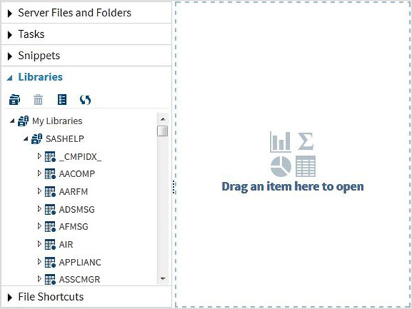
SAS Built-In Data Sets

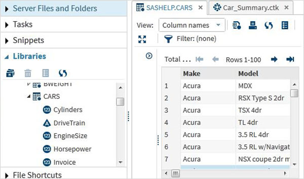
These Data Sets are already available in the installed SAS software. They can be explored and used in formulating sample expressions for data analysis. To explore these data sets go to Libraries -> My Libraries -> SASHELP. On expanding it we see the list of names of all the built-in Data Sets available.

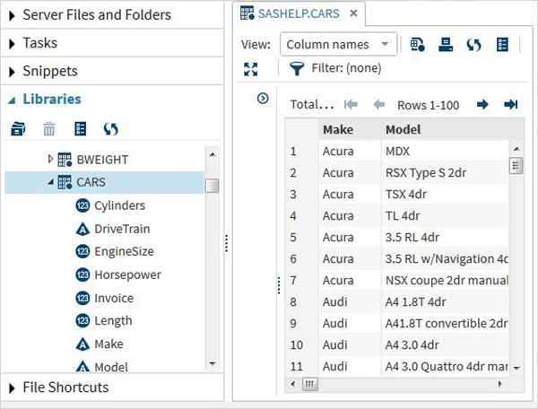
Lets scroll down to locate a Data Set named CARS.Double clicking on this Data Set opens it in the right window pane where we can explore it further.We can also minimize the left pane by using the maximize view button under the right pane.

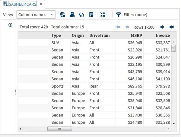
We can scroll to the right using the scroll bar in the bottom to explore all the columns and theirs values in the table.

Importing External Data Sets

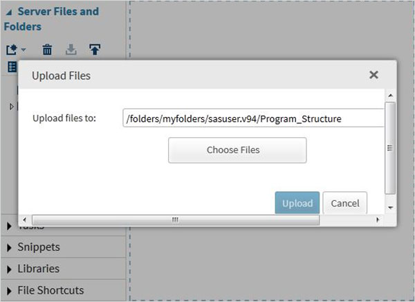
We can export our own files as Data sets by using the import feature available in SAS Studio. But these files must be available in the SAS server folders. So we have to upload the source data files to SAS folder by using the upload option under the Server Files and Folders.

Next we use the above file in a SAS program by importing it. To do this we use the option Tasks -> Utilities -> Import data as shown below. Double click the Import Data button which opens up the window in the right to choose the file for the Data Set.

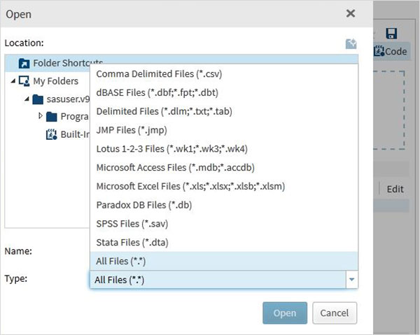
Next Click on the Select Files button under the import data program in the right pane. The following are the list of the file types which can be imported.

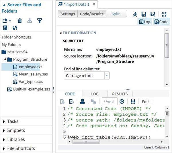
We choose the "employee.txt" file stored in the local system and get the file imported as shown below.

View the imported data

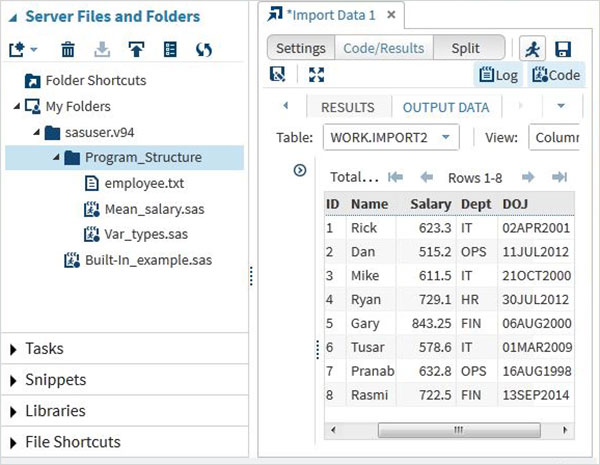
We can view the imported data by running the default import code generated using the Run option

We can import any other file types using the same approach as above and use it in various SAS programs.

SAS - Variables

In general variables in SAS represent the column names of the data tables it is analysing. But it can also be used for other purpose like using it as a counter in a programming loop. In the current chapter we will see the use of SAS variables as column names of SAS Data Set.

SAS Variable Types

SAS has three types of variables as below −

Numeric Variables

This is the default variable type. These variables are used in mathematical expressions.

Syntax

INPUT VAR1 VAR2 VAR3; 		#Define numeric variables in the data set.

In the above syntax, the INPUT statement shows the declaration of numeric variables.

Example

INPUT ID SALARY COMM_PERCENT;

Character Variables

Character variables are used for values that are not used in Mathematical expressions. They are treated as text or strings. A variable becomes a character variable by adding a $ sing with a space at the end of the variable name.

Syntax

INPUT VAR1 $ VAR2 $ VAR3 $; 	#Define character variables in the data set.

In the above syntax, the INPUT statement shows the declaration of character variables.

Example

INPUT FNAME $ LNAME $ ADDRESS $;

Date Variables

These variables are treated only as dates and they need to be in valid date formats. A variable becomes a date variable by adding a date format with a space at the end of the variable name.

Syntax

INPUT VAR1 DATE11. VAR2 MMDDYY10. ; #Define date variables in the data set.

In the above syntax, the INPUT statement shows the declaration of date variables.

Example

INPUT DOB DATE11. START_DATE MMDDYY10. ;

Use of Variables in SAS Program

The above variables are used in SAS program as shown in below examples.

Example

The below code shows how the three types of variables are declared and used in a SAS Program

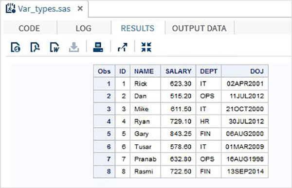
DATA TEMP;
INPUT ID NAME $ SALARY DEPT $ DOJ DATE9. ;
FORMAT DOJ DATE9. ;
DATALINES;
1 Rick 623.3 IT 02APR2001
2 Dan 515.2 OPS 11JUL2012
3 Michelle 611 IT 21OCT2000
4 Ryan 729 HR 30JUL2012
5 Gary 843.25 FIN 06AUG2000
6 Tusar 578 IT 01MAR2009
7 Pranab 632.8 OPS 16AUG1998
8 Rasmi 722.5 FIN 13SEP2014
;
PROC PRINT DATA = TEMP;
RUN;

In the above example all the character variables are declared followed by a $ sign and the date variables are declared followed by a date format. The output of the above program is as below.

Using the Variables

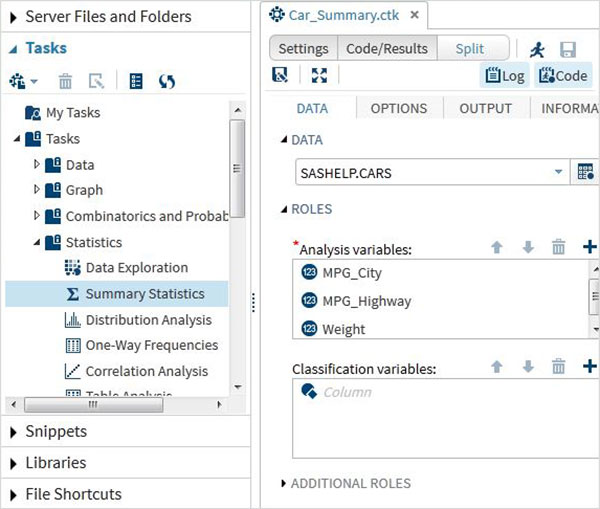
The variables are very useful in analysing the data. They are used in expressions in which the statistical analysis is applied. Let’s see an example of analysing the built-in Data Set named CARS which is present under Libraries → My Libraries → SASHELP. Double click on it to explore the variables and their data types.

Next we can produce a summary statistics of some of these variables using the Tasks options in SAS studio. Go to Tasks -> Statistics -> Summary Statistics and double click it to open the window as shown below. Choose Data Set SASHELP.CARS and select the three variables - MPG_CITY, MPG_Highway and Weight under the Analysis Variables. Hold the Ctrl key while selecting the variables by clicking. Click run.

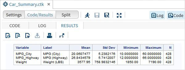
Click on the results tab after the above steps. It shows the statistical summary of the three variables chosen. The last column indicates number of observations (records) used in the analysis.

SAS - Strings

Strings in SAS are the values which are enclosed with in a pair of single quotes. Also the string variables are declared by adding a space and $ sign at the end of the variable declaration. SAS has many powerful functions to analyze and manipulate strings.

Declaring String Variables

We can declare the string variables and their values as shown below. In the code below we declare two character variables of lengths 6 and 5. The LENGTH keyword is used for declaring variables without creating multiple observations.

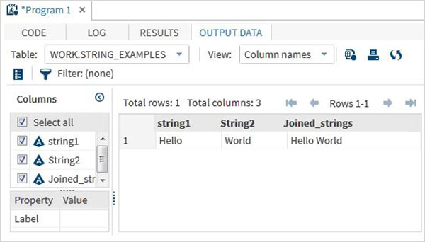
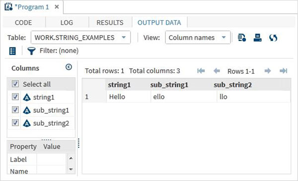
data string_examples;
   LENGTH string1 $ 6 String2 $ 5;
   /*String variables of length 6 and 5 */
   String1 = 'Hello';
   String2 = 'World';
   Joined_strings =  String1 ||String2 ;
run;
proc print data = string_examples noobs;
run;

On running the above code we get the output which shows the variable names and their values.

String Functions

Below are the examples of some SAS functions which are used frequently.

SUBSTRN

This function extracts a substring using the start and end positions. In case of no end position is mentioned it extracts all the characters till end of the string.

Syntax

SUBSTRN('stringval',p1,p2)

Following is the description of the parameters used −

stringval is the value of the string variable.
p1 is the start position of extraction.
p2 is the final position of extraction.

Example

data string_examples;
   LENGTH string1 $ 6 ;
   String1 = 'Hello';
   sub_string1 = substrn(String1,2,4) ;
   /*Extract from position 2 to 4 */
   sub_string2 = substrn(String1,3) ;
   /*Extract from position 3 onwards */
run;
proc print data = string_examples noobs;
run;

On running the above code we get the output which shows the result of substrn function.

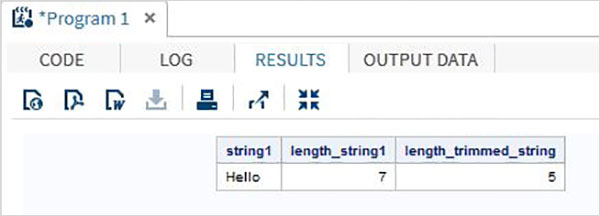
TRIMN

This function removes the trailing space form a string.

Syntax

TRIMN('stringval')

Following is the description of the parameters used −

stringval is the value of the string variable.

data string_examples;
   LENGTH string1 $ 7  ;
   String1='Hello  ';
   length_string1 = lengthc(String1);
   length_trimmed_string = lengthc(TRIMN(String1));
run;
proc print data = string_examples noobs;
run;

On running the above code we get the output which shows the result of TRIMN function.

SAS - Arrays

Arrays in SAS are used to store and retrieve a series of values using an index value. The index represents the location in a reserved memory area.

Syntax

In SAS an array is declared by using the following syntax −

ARRAY ARRAY-NAME(SUBSCRIPT) ($) VARIABLE-LIST ARRAY-VALUES

In the above syntax −

ARRAY is the SAS keyword to declare an array.
ARRAY-NAME is the name of the array which follows the same rule as variable names.
SUBSCRIPT is the number of values the array is going to store.
($) is an optional parameter to be used only if the array is going to store character values.
VARIABLE-LIST is the optional list of variables which are the place holders for array values.
ARRAY-VALUES are the actual values that are stored in the array. They can be declared here or can be read from a file or dataline.

Examples of Array Declaration

Arrays can be declared in many ways using the above syntax. Below are the examples.

# Declare an array of length 5 named AGE with values.
ARRAY AGE[5] (12 18 5 62 44);

# Declare an array of length 5 named COUNTRIES with values starting at index 0.
ARRAY COUNTRIES(0:8) A B C D E F G H I;

# Declare an array of length 5 named QUESTS which contain character values.
ARRAY QUESTS(1:5) $ Q1-Q5;

# Declare an array of required length as per the number of values supplied.
ARRAY ANSWER(*) A1-A100;

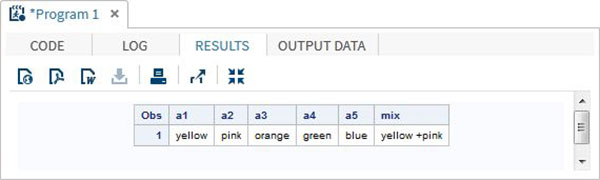
Accessing Array Values

The values stored in an array can be accessed by using the print procedure as shown below. After it is declared using one of the above methods, the data is supplied using DATALINES statement.

DATA array_example;
INPUT a1 $ a2 $ a3 $ a4 $ a5 $;
ARRAY colours(5) $ a1-a5;
mix = a1||'+'||a2;
DATALINES;
yello pink orange green blue
;
RUN;
PROC PRINT DATA = array_example;
RUN;

When we execute above code, it produces following result −

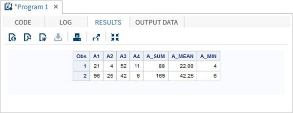
Using the OF operator

The OF operator is used when analysing the data forma an Array to perform calculations on the entire row of an array. In the below example we apply the Sum and Mean of values in each row.

DATA array_example_OF;
   INPUT A1 A2 A3 A4;
   ARRAY A(4) A1-A4;
   A_SUM = SUM(OF A(*));
   A_MEAN = MEAN(OF A(*));
   A_MIN = MIN(OF A(*));
   DATALINES;
   21 4 52 11
   96 25 42 6
   ;
   RUN;
   PROC PRINT DATA = array_example_OF;
   RUN;

When we execute above code, it produces following result −

Using the IN operator

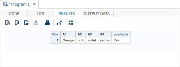
The value in an array can also be accessed using the IN operator which checks for the presence of a value in the row of the array. In the below example we check for the availability of the colour "Yellow" in the data. This value is case sensitive.

DATA array_in_example;
   INPUT A1 $ A2 $ A3 $ A4 $;
   ARRAY COLOURS(4) A1-A4;
   IF 'yellow' IN COLOURS THEN available = 'Yes';ELSE available = 'No';
   DATALINES;
   Orange pink violet yellow
   ;
   RUN;
   PROC PRINT DATA = array_in_example;
   RUN;

When we execute above code, it produces following result −

SAS - Numeric Formats

SAS can handle a wide variety of numeric data formats. It uses these formats at the end of the variable names to apply a specific numeric format to the data. SAS use two kinds of numeric formats. One for reading specific formats of the numeric data which is called informat and another for displaying the numeric data in specific format called as output format.

Syntax

The Syntax for a numeric informat is −

Varname Formatnamew.d

Following is the description of the parameters used −

Varname is the name of the variable.
Formatname is the name of the name of the numeric format applied to the variable.
w is the maximum number of data columns (including digits after decimal & the decimal point itself) allowed to be stored for the variable.
d is the number of digits to the right of the decimal.

Reading Numeric formats

Below is a list of formats used for reading the data into SAS.

Input Numeric Formats

Format	Use
n.	Maximum "n" number of columns with no decimal point.
n.p	Maximum "n" number of columns with "p" decimal points.
COMMAn.p	Maximum "n" number of columns with "p" decimal places which removes any comma or dollar signs.
COMMAn.p	Maximum "n" number of columns with "p" decimal places which removes any comma or dollar signs.

Displaying Numeric formats

Similar to applying format while reading the data, below is a list of formats used for displaying the data in the output of a SAS program.

Output Numeric Formats

Format	Use
n.	Write maximum "n" number of digits with no decimal point.
n.p	Write maximum "n.p" number of columns with "p" decimal points.
DOLLARn.p	Write maximum "n" number of columns with p decimal places, leading dollar sign and a comma at the thousandth place.

Please Note −

If the number of digits after the decimal point is less than the format specifier thenzeros will be appended at the end.
If the number of digits after the decimal point is greater than the format specifier then the last digit will be rounded off.

Examples

Below examples illustrate above scenarios.

DATA MYDATA1;
input x 6.; /*maxiiuum width of the data*/
format x 6.3;
datalines;
8722
93.2
.1122
15.116
PROC PRINT DATA = MYDATA1;
RUN;

DATA MYDATA2;
input x 6.; /*maximum width of the data*/
format x 5.2;
datalines;
8722
93.2
.1122
15.116
PROC PRINT DATA = MYDATA2;
RUN;
DATA MYDATA3;
input x 6.; /*maximum width of the data*/
format x DOLLAR10.2;
datalines;
8722
93.2
.1122
15.116
PROC PRINT DATA = MYDATA3;
RUN;

When we execute above code, it produces following result −

# MYDATA1.
Obs 	x
1 	8722.0 # Display 6 columns with zero appended after decimal.
2 	93.200 # Display 6 columns with zero appended after decimal.
3 	0.112  # No integers before decimal, so display 3 available digits after decimal.
4 	15.116 # Display 6 columns with 3 available digits after decimal.

# MYDATA2
Obs 	x
1 	8722  # Display 5 columns. Only 4 are available.
2 	93.20 # Display 5 columns with zero appended after decimal.
3 	0.11  # Display 5 columns with 2 places after decimal.
4 	15.12 # Display 5 columns with 2 places after decimal.

# MYDATA3
Obs 	x
1 	$8,722.00 # Display 10 columns with leading $ sign, comma at thousandth place and zeros appended after decimal.
2 	$93.20    # Only 2 integers available before decimal and one available after the decimal.
3 	$0.11	  # No integers available before decimal and two available after the decimal.
4 	$15.12    # Only 2 integers available before decimal and two available after the decimal.

SAS - Operators

An operator in SAS is a symbol which is used in a mathematical, logical or comparison expression. These symbols are in-built into the SAS language and many operators can be combined in a single expression to give a final output.

Below is a list of SAS category of operators.

Arithmetic Operators
Logical Operators
Comparison Operators
Minimum/Maximum Operators
Concatenation Operator

We will look at each of the one by one. The operators are always used with variables that are part of the data that is being analyzed by the SAS program.

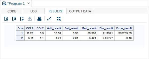
Arithmetic Operators

The below table describes the details of the arithmetic operators. Let’s assume two data variables V1 and V2with values 8 and 4 respectively.

Operator	Description	Example
+	Addition	V1+V2=12
-	Subtraction	V1-V2=4
*	Multiplication	V1*V2=32
/	Division	V1/V2=2
**	Exponentiation	V1**V2=4096

Example

DATA MYDATA1;
input @1 COL1 4.2	@7 COL2 3.1; 
Add_result = COL1+COL2;
Sub_result = COL1-COL2;
Mult_result = COL1*COL2;
Div_result = COL1/COL2;
Expo_result = COL1**COL2;
datalines;
11.21 5.3
3.11  11
;
PROC PRINT DATA = MYDATA1;
RUN;

On running the above code, we get the following output.

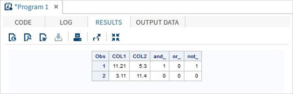
Logical Operators

The below table describes the details of the logical operators. These operators evaluate the Truth value of an expression. So the result of logical operators is always a 1 or a 0. Let’s assume two data variables V1 and V2with values 8 and 4 respectively.

Operator	Description	Example
&	The AND Operator. If both data values evaluate to true then the result is 1 else it is 0.	(V1>2 & V2 > 3) gives 0.
\|	The OR Operator. If any one of the data values evaluate to true then the result is 1 else it is 0.	(V1>9 & V2 > 3) is 1.
~	The NOT Operator. The result of NOT operator in form of an expression whose value is FALSE or a missing value is 1 else it is 0.	NOT(V1 > 3) is 1.

Example

DATA MYDATA1;
input @1 COL1 5.2	@7 COL2 4.1; 
and_=(COL1 > 10 & COL2 > 5 );
or_ = (COL1 > 12 | COL2 > 15 );
not_ = ~( COL2 > 7 );
datalines;
11.21 5.3
3.11  11.4
;
PROC PRINT DATA = MYDATA1;
RUN;

On running the above code, we get the following output.

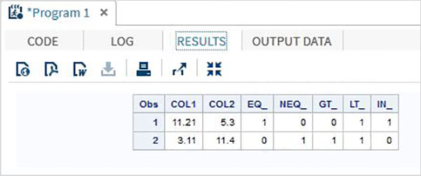
Comparison Operators

The below table describes the details of the comparison operators. These operators compare the values of the variables and the result is a truth value presented by 1 for TRUE and 0 for False. Let’s assume two data variables V1 and V2with values 8 and 4 respectively.

Operator	Description	Example
=	The EQUAL Operator. If both data values are equal then the result is 1 else it is 0.	(V1 = 8) gives 1.
^=	The NOT EQUAL Operator. If both data values are unequal then the result is 1 else it is 0.	(V1 ^= V2) gives 1.
<	The LESS THAN Operator.	(V2 < V2) gives 1.
<=	The LESS THAN or EQUAL TO Operator.	(V2 <= 4) gives 1.
>	The GREATER THAN Operator.	(V2 > V1) gives 1.
>=	The GREATER THAN or EQUAL TO Operator.	(V2 >= V1) gives 0.
IN	The IN Operator. If the value of the variable is equal to any one of the values in a given list of values, then it returns 1 else it returns 0.	V1 in (5,7,9,8) gives 1.

Example

DATA MYDATA1;
input @1 COL1 5.2	@7 COL2 4.1; 
EQ_ = (COL1 = 11.21);
NEQ_= (COL1 ^= 11.21);
GT_ = (COL2 => 8);
LT_ = (COL2 <= 12);
IN_ = COL2 in( 6.2,5.3,12 );
datalines;
11.21 5.3
3.11  11.4
;
PROC PRINT DATA = MYDATA1;
RUN;

On running the above code, we get the following output.

Minimum/Maximum Operators

The below table describes the details of the Minimum/Maximum operators. These operators compare the values of the variables across a row and the minimum or maximum value from the list of values in the rows is returned.

Operator	Description	Example
MIN	The MIN Operator. It returns the minimum value form the list of values in the row.	MIN(45.2,11.6,15.41) gives 11.6
MAX	The MAX Operator. It returns the maximum value form the list of values in the row.	MAX(45.2,11.6,15.41) gives 45.2

Example

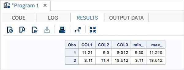
DATA MYDATA1;
input @1 COL1 5.2	@7 COL2 4.1 @12 COL3 6.3; 
min_ = MIN(COL1 , COL2 , COL3);
max_ = MAX( COL1, COl2 , COL3);
datalines;
11.21 5.3 29.012
3.11  11.4 18.512
;
PROC PRINT DATA = MYDATA1;
RUN;

On running the above code, we get the following output.

Concatenation Operator

The below table describes the details of the Concatenation operator. This operator concatenates two or more string values. A single character value is returned.

Operator	Description	Example
\|\|	The concatenate Operator. It returns the concatenation of two or more values.	'Hello'\|\|' World' gives Hello World

Example

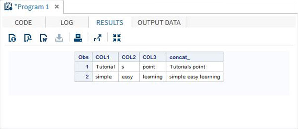
DATA MYDATA1;
input  COL1 $	COL2 $  COL3 $; 
concat_ = (COL1 || COL2 || COL3);
datalines;
Tutorial s point
simple easy learning
;
PROC PRINT DATA = MYDATA1;
RUN;

On running the above code, we get the following output.

Operators Precedence

The operator precedence indicates the order of evaluation of the multiple operators present in complex expression. The below table describes the order of precedence with in a group of operators.

Group	Order	Symbols
Group I	Right to Left	** + - NOT MIN MAX
Group II	Left to Right	* /
Group III	Left to Right	+ -
Group IV	Left to Right	\|\|
Group V	Left to Right	< <= = >= >

SAS - Loops

You may encounter situations, when a block of code needs to be executed several number of times. In general, statements are executed sequentially − The first statement in a function is executed first, followed by the second, and so on. But when you want the same set of statements to be executed again and again, we need the help of Loops.

In SAS looping is done by using DO statement. It is also called DO Loop. Given below is the general form of a DO loop statements in SAS.

Flow Diagram

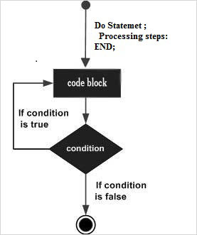
Following are the types of DO loops in SAS.

Sr.No.	Loop Type & Description
1	DO Index. The loop continues from the start value till the stop value of the index variable.
2	DO WHILE. The loop continues till the while condition becomes false.
3	DO UNTIL. The loop continues till the UNTIL condition becomes True.

SAS - Decision Making

Decision making structures require the programmer to specify one or more conditions to be evaluated or tested by the program, along with a statement or statements to be executed if the condition is determined to be true, and optionally, other statements to be executed if the condition is determined to be false.

Following is the general form of a typical decision making structure found in most of the programming languages −

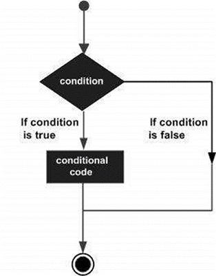
SAS provides following types of decision making statements. Click the following links to check their detail.

Sr.No.	Statement Type & Description
1	IF Statement. An if statement consists of a condition. If the condition is true then the specific data is fetched.
2	IF-THEN-ELSE Statement. An if statement followed by else statement, which executes when the boolean condition is false.
3	IF-THEN-ELSE-IF Statement. An if statement followed by else statement, which is again followed by another pair of IF-THEN Statement.
4	IF-THEN-DELETE Statement. An if statement consists of acondition, which when true deletes the specific data from the observations.

SAS - Functions

SAS has a wide variety of in built functions which help in analysing and processing the data. These functions are used as part of the DATA statements. They take the data variables as arguments and return the result which is stored into another variable. Depending on the type of function, the number of arguments it takes can vary. Some functions accept zero arguments while some other accept fixed number of variables. Below is a list of types of functions SAS provides.

Syntax

The general syntax for using a function in SAS is as below.

FUNCTIONNAME(argument1, argument2...argumentn)

Here the argument can be a constant, variable, expression or another function.

Function Categories

Depending on their usage, the functions in SAS are categorised as below.

Mathematical
Date and Time
Character
Truncation
Miscellaneous

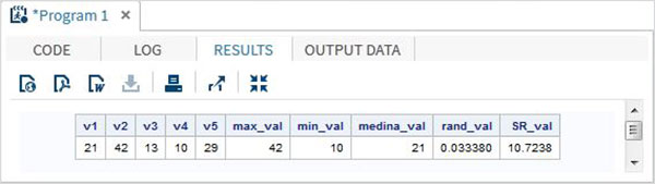
Mathematical Functions

These are the functions used to apply some mathematical calculations on the variable values.

Examples

The below SAS program shows the use of some important mathematical functions.

data Math_functions;

v1=21; v2=42; v3=13; v4=10; v5=29;

/* Get Maximum value */
max_val = MAX(v1,v2,v3,v4,v5);

/* Get Minimum value */
min_val = MIN (v1,v2,v3,v4,v5);

/* Get Median value */
med_val = MEDIAN (v1,v2,v3,v4,v5);

/* Get a random number */
rand_val = RANUNI(0);

/* Get Square root of sum of the values */
SR_val= SQRT(sum(v1,v2,v3,v4,v5));

proc print data = Math_functions noobs;
run;

When the above code is run, we get the following output −

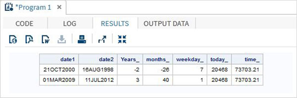
Date and Time Functions

These are the functions used to process date and time values.

Examples

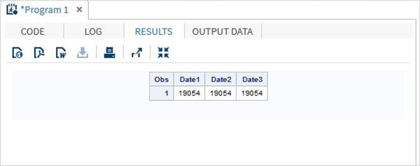
The below SAS program shows the use of date and time functions.

data date_functions;
INPUT @1 date1 date9. @11 date2 date9.;
format date1 date9.  date2 date9.;

/* Get the interval between the dates in years*/
Years_ = INTCK('YEAR',date1,date2);

/* Get the interval between the dates in months*/
months_ = INTCK('MONTH',date1,date2);

/* Get the week day from the date*/
weekday_ =  WEEKDAY(date1);

/* Get Today's date in SAS date format */
today_ = TODAY();

/* Get current time in SAS time format */
time_ = time();
DATALINES;
21OCT2000 16AUG1998
01MAR2009 11JUL2012
;
proc print data = date_functions noobs;
run;

When the above code is run, we get the following output −

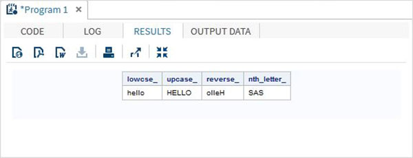
Character Functions

These are the functions used to process character or text values.

Examples

The below SAS program shows the use of character functions.

data character_functions;

/* Convert the string into lower case */
lowcse_ = LOWCASE('HELLO');
  
/* Convert the string into upper case */
upcase_ = UPCASE('hello');
  
/* Reverse the string */
reverse_ = REVERSE('Hello');
  
/* Return the nth word */
nth_letter_ = SCAN('Learn SAS Now',2);
run;

proc print data = character_functions noobs;
run;

When the above code is run, we get the following output −

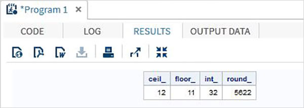
Truncation Functions

These are the functions used to truncate numeric values.

Examples

The below SAS program shows the use of truncation functions.

data trunc_functions;

/* Nearest greatest integer */
ceil_ = CEIL(11.85);
  
/* Nearest greatest integer */
floor_ = FLOOR(11.85);
  
/* Integer portion of a number */
int_ = INT(32.41);
  
/* Round off to nearest value */
round_ = ROUND(5621.78);
run;

proc print data = trunc_functions noobs;
run;

When the above code is run, we get the following output −

Miscellaneous Functions

Let us now understand the miscellaneous functions of SAS with some examples.

Examples

The below SAS program shows the use of Miscellaneous functions.

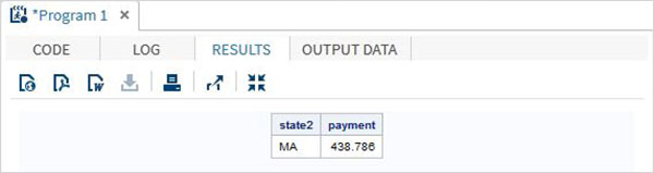
data misc_functions;

/* Nearest greatest integer */
state2=zipstate('01040');
 
/* Amortization calculation */
payment = mort(50000, . , .10/12,30*12);

proc print data = misc_functions noobs;
run;

When the above code is run, we get the following output −

SAS - Input Methods

The input methods are used to read the raw data. The raw data may be from an external source or from in stream datalines. The input statement creates a variable with the name that you assign to each field. So you have to create a variable in the Input Statement. The same variable will be shown in the output of SAS Dataset. Below are different input methods available in SAS.

List Input Method
Named Input Method
Column Input Method
Formatted Input Method

The details of each input method is described as below.

List Input Method

In this method the variables are listed with the data types. The raw data is carefully analysed so that the order of the variables declared matches the data. The delimiter (usually space) should be uniform between any pair of adjacent columns. Any missing data will cause problem in the output as the result will be wrong.

Example

The following code and the output shows the use of list input method.

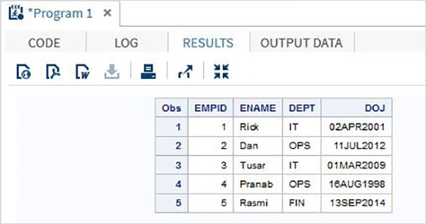
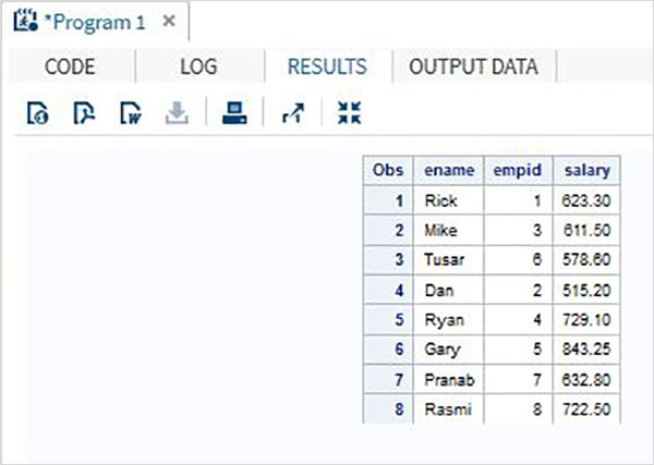
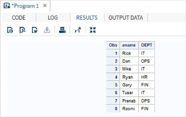
DATA TEMP;
INPUT   EMPID ENAME $ DEPT $ ;
DATALINES;
1 Rick  IT
2 Dan  OPS
3 Tusar  IT
4 Pranab  OPS
5 Rasmi  FIN
;
PROC PRINT DATA = TEMP;
RUN;

On running the bove code we get the following output.

Named Input Method

In this method the variables are listed with the data types. The raw data is modified to have variable names declared in front of the matching data. The delimiter (usually space) should be uniform between any pair of adjacent columns.

Example

The following code and the output show the use of Named Input Method.

DATA TEMP;
INPUT   
EMPID= ENAME= $ DEPT= $ ;
DATALINES;
EMPID = 1 ENAME = Rick  DEPT = IT
EMPID = 2 ENAME = Dan  DEPT = OPS
EMPID = 3 ENAME = Tusar  DEPT = IT
EMPID = 4 ENAME = Pranab  DEPT = OPS
EMPID = 5 ENAME = Rasmi  DEPT = FIN
;
PROC PRINT DATA = TEMP;
RUN;

On running the bove code we get the following output.

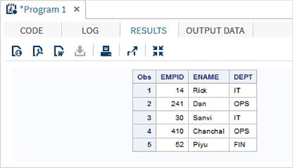
Column Input Method

In this method the variables are listed with the data types and width of the columns which specify the value of the single column of data. For example if an employee name contains maximum 9 characters and each employee name starts at 10th column, then the column width for employee name variable will be 10-19.

Example

Following code shows the use of Column Input Method.

DATA TEMP;
INPUT   EMPID 1-3 ENAME $ 4-12 DEPT $ 13-16;
DATALINES;
14 Rick     IT 
241Dan      OPS 
30 Sanvi    IT 
410Chanchal OPS 
52 Piyu     FIN 
;
PROC PRINT DATA = TEMP;
RUN;

When we execute above code, it produces following result −

Formatted Input Method

In this method the variables are read from a fixed starting point until a space is encountered. As every variable has a fixed starting point, the number of columns between any pair of variables becomes the width of the first variable. The character '@n' is used to specify the starting column position of a variable as the nth column.

Example

The following code shows the use of Formatted Input Method

DATA TEMP;
INPUT   @1 EMPID $ @4 ENAME $ @13 DEPT $ ;
DATALINES;
14 Rick     IT 
241 Dan      OPS 
30 Sanvi    IT 
410 Chanchal OPS 
52 Piyu     FIN 
;
PROC PRINT DATA = TEMP;
RUN;

When we execute above code, it produces following result −

SAS - Macros

SAS has a powerful programming feature called Macros which allows us to avoid repetitive sections of code and to use them again and again when needed. It also helps create dynamic variables within the code that can take different values for different run instances of the same code. Macros can also be declared for blocks of code which will be reused multiple times in a similar manner to macro variables. We will see both of these in the below examples.

Macro variables

These are the variables which hold a value to be used again and again by a SAS program. They are declared at the beginning of a SAS program and called out later in the body of the program. They can be Global or Local in scope.

Global Macro variable

They are called global macro variables because they can accessed by any SAS program available in the SAS environment. In general they are the system assigned variables which are accessed by multiple programs. A general example is the system date.

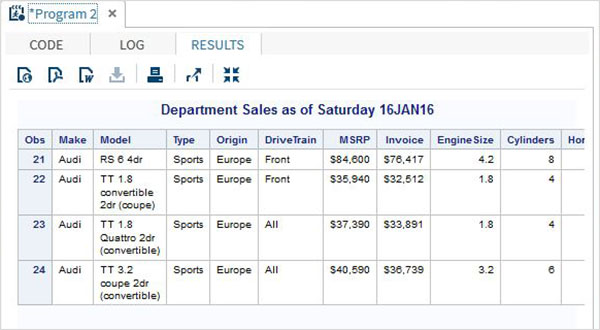
Example

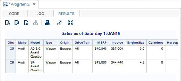
Below is a example of the SAS variable called SYSDATE which represents the system date. Consider a scenario to print the system date in the title of the SAS report every day the report is generated. The title will show the current date and day without we coding any values for them. We use the in-built SAS data set called CARS available in the SASHELP library.

proc print data = sashelp.cars;
where make = 'Audi' and type = 'Sports' ;
 TITLE "Sales as of &SYSDAY &SYSDATE";
run;

When the above code is run we get the following output.

Local Macro variable

These variables can be accessed by SAS programs in which they are declared as part of the program. They are typically used to supply different varaibels to the same SAS statements sl that they can process different observations of a data set.

Syntax

The local variables are decalred with below syntax.

% LET (Macro Variable Name) = Value;

Here the Value field can take any numeric, text or date value as required by the program. The Macro variable name is any valid SAS variable.

Example

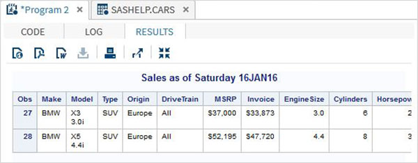
The variables are used by the SAS statements using the & character appended at the beginning of the variable name. Below program gets us all the observation of the make 'Audi' and type 'Sports'. In case we want the result of different make, we need to change the value of the variable make_name without changing any other part of the program. In case of bring programs this variable can be referred again and again in any SAS statements.

%LET make_name = 'Audi';
%LET type_name = 'Sports';
proc print data = sashelp.cars;
where make = &make_name and type = &type_name ;
 TITLE "Sales as of &SYSDAY &SYSDATE";
run;

When the above code is run we get the same output as the previous program. But let’s change the type name to 'Wagon' and run the same program. We will get the below result.

Macro Programs

Macro is a group of SAS statements that is referred by a name and to use it in program anywhere, using that name. It starts with a %MACRO statement and ends with %MEND statement.

Syntax

The local variables are declared with below syntax.

# Creating a Macro program.
%MACRO <macro name>(Param1, Param2,….Paramn);

Macro Statements;

%MEND;

# Calling a Macro program.
%MacroName (Value1, Value2,…..Valuen);

Example

The below program decalres a group of SAT staemnets under a macro named 'show_result'; This Macro is being called by other SAS statements.

%MACRO show_result(make_ , type_);
proc print data = sashelp.cars;
where make = "&make_" and type = "&type_" ;
TITLE "Sales as of &SYSDAY &SYSDATE";
run;
%MEND;

%show_result(BMW,SUV);

When the above code is run we get the following output.

Commonly Used Macros

SAS has many MACRO statements which are in-built in the SAS programming language. They are used by other SAS programs without explicitly declaring them.Common examples are - terminating a program when some condition is met or capturing the runtime value of a variable in the program log. Below are some examples.

Macro %PUT

This macro statement writes text or macro variable information to the SAS log. In the below example the value of the variable 'today' is written to the program log.

data _null_;
CALL SYMPUT ('today',
TRIM(PUT("&sysdate"d,worddate22.)));
run;
%put &today;

When the above code is run we get the following output.

Macro %RETURN

Execution of this macro causes normal termination of the currently executing macro when certain condition evaluates to be true. In the below examplewhen the value of the variable "val" becomes 10, the macro terminates else it contnues.

%macro check_condition(val);
   %if &val = 10 %then %return;

   data p;
      x = 34.2;
   run;  

%mend check_condition;  

%check_condition(11)  ;

When the above code is run we get the following output.

Macro %END

This macro definition contains a %DO %WHILE loop that ends, as required, with a %END statement. In the below example the macro named test takes a user input and runs the DO loop using this input value. The end of DO loop is achieved through the %end statement while the end of macro is achieved through %mend statement.

%macro test(finish);
   %let i = 1;
   %do %while (&i <&finish);
      %put the value of i is &i;
      %let i=%eval(&i+1);
   %end;
%mend test;
%test(5)

When the above code is run we get the following output.

SAS - Date & Times

IN SAS dates are a special case of numeric values. Each day is assigned a specific numeric value starting from 1st January 1960. This date is assigned the date value 0 and the next date has a date value of 1 and so on. The previous days to this date are represented by -1 , -2 and so on. With this approach SAS can represent any date in future and any date in past.

When SAS reads the data from a source it converts the data read into a specific date format as specified the date format. The variable to store the date value is declared with the proper informat required. The output date is shown by using the output data formats.

SAS Date Informat

The source data can be read properly by using specific date informats as shown below. The digit at the end of the informat indicates the minimum width of the date string to be read completely using the informat. A smaller width will give incorrect result. with SAS V9, there is a generic date format anydtdte15. which can process any date input.

Input Date	Date width	Informat
03/11/2014	10	mmddyy10.
03/11/14	8	mmddyy8.
December 11, 2012	20	worddate20.
14mar2011	9	date9.
14-mar-2011	11	date11.
14-mar-2011	15	anydtdte15.

Example

The below code shows the reading of different date formats. Please note the all the output values are just numbers as we have not applied any format statement to the output values.

DATA TEMP;
INPUT @1 Date1 date11. @12 Date2 anydtdte15. @23 Date3 mmddyy10.   ;
DATALINES;
02-mar-2012 3/02/2012 3/02/2012
;
PROC PRINT DATA = TEMP;
RUN;

When the above code is executed, we get the following output.

SAS Date output format

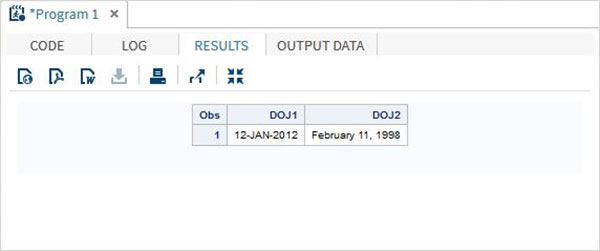
The dates after being read , can be converted to another format as required by the display. This is achieved using the format statement for the date types. They take the same formats as informats.

Example

In the below exampel the date is read in one format but displayed in another format.

DATA TEMP;
INPUT  @1 DOJ1 mmddyy10. @12 DOJ2 mmddyy10.;
format  DOJ1 date11.  DOJ2 worddate20. ;
DATALINES;
01/12/2012 02/11/1998 
;
PROC PRINT DATA = TEMP;
RUN;

When the above code is executed, we get the following output.

SAS - Read Raw Data

SAS can read data from various sources which includes many file formats. The file formats used in SAS environment is discussed below.

ASCII(Text) Data Set
Delimited Data
Excel Data
Hierarchical Data

Reading ASCII(Text) Data Set

These are the files which contain the data on text format. The data is usually delimited by a space, but there can be different types of delimiters also which SAS can handle. Let’s consider an ASCII file containing the employee data. We read this file using the Infile statement available in SAS.

Example

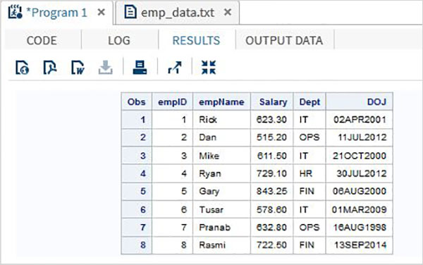
In the below example we read the data file named emp_data.txt from the local environment.

data TEMP; 
   infile 
   '/folders/myfolders/sasuser.v94/TutorialsPoint/emp_data.txt'; 
   input empID empName $ Salary Dept $ DOJ date9. ;
   format DOJ date9.;
   run;
   PROC PRINT DATA = TEMP;
RUN;

When the above code is executed, we get the following output.

Reading Delimited Data

These are the data files in which the column values are separated by a delimiting character like a comma or pipeline etc. In this case we use the dlm option in the infile statement.

Example

In the below example we read the data file named emp.csv from the local environment.

data TEMP; 
   infile 
   '/folders/myfolders/sasuser.v94/TutorialsPoint/emp.csv' dlm=","; 
   input empID empName $ Salary Dept $ DOJ date9. ;
   format DOJ date9.;
   run;
   PROC PRINT DATA = TEMP;
RUN;

When the above code is executed, we get the following output.

Reading Excel Data

SAS can directly read an excel file using the import facility. As seen in the chapter SAS data sets, it can handle a wide variety of file types including MS excel. Assuming the file emp.xls is available locally in the SAS environment.

Example

FILENAME REFFILE
"/folders/myfolders/TutorialsPoint/emp.xls"
TERMSTR = CR;

PROC IMPORT DATAFILE = REFFILE
DBMS = XLS
OUT = WORK.IMPORT;
GETNAMES = YES;
RUN;
PROC PRINT DATA = WORK.IMPORT RUN;

The above code reads the data from excel file and gives the same output as above two file types.

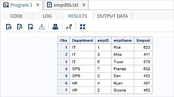
Reading Hierarchical Files

In these files the data is present in hierarchical format. For a given observation there is a header record below which many detail records are mentioned. The number of details records can vary from one observation to another. Below is an illustration of a hierarchical file.

In the below file the details of each employee under each department is listed. The first record is the header record mentioning the department and the next record few records starting with DTLS are the details record.

DEPT:IT 
DTLS:1:Rick:623 
DTLS:3:Mike:611 
DTLS:6:Tusar:578 
DEPT:OPS
DTLS:7:Pranab:632
DTLS:2:Dan:452
DEPT:HR
DTLS:4:Ryan:487
DTLS:2:Siyona:452

Example

To read the hierarchical file we use the below code in which we identify the header record with an IF clause and use a do loop to process the details record.

data employees(drop = Type);
   length Type $ 3  Department
      empID $ 3 empName $ 10 Empsal 3 ;
   retain Department;
   infile 
   '/folders/myfolders/TutorialsPoint/empdtls.txt' dlm = ':';
   input Type $ @;
   if Type = 'DEP' then 
      input Department $;
   else do;
      input empID  empName $ Empsal ;
      output;
   end;
run;

   PROC PRINT DATA = employees;
RUN;

When the above code is executed, we get the following output.

SAS - Write Data Sets

Similar to reading datasets, SAS can write datasets in different formats. It can write data from SAS files to normal text file.These files can be read by other software programs. SAS uses PROC EXPORT to write data sets.

PROC EXPORT

It is a SAS inbuilt procedure used to export the SAS data sets for writing the data into files of different formats.

Syntax

The basic syntax for writing the procedure in SAS is −

PROC EXPORT 
DATA = libref.SAS data-set (SAS data-set-options)
OUTFILE = "filename" 
DBMS = identifier LABEL(REPLACE);

Following is the description of the parameters used −

SAS data-set is the data set name which is being exported. SAS can share the data sets from its environment with other applications by creating files which can be read by different operating systems. It uses the inbuilt EXPORT function to out the data set files in a variety of formats. In this chapter we will see the writing of SAS data sets using proc export along with the options dlm and dbms.
SAS data-set-options is used to specify a subset of columns to be exported.
filename is the name of the file to which the data is written into.
identifier is used to mention the delimiter that will be written into the file.
LABEL option is used to mention the name of the variables written to the file.

Example

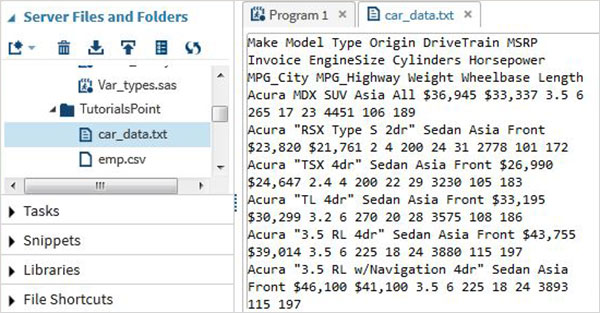
We will use the SAS data set named cars available in the SASHELP library. We export it as a space delimited text file with the code as shown in the following program.

proc export data = sashelp.cars
   outfile = '/folders/myfolders/sasuser.v94/TutorialsPoint/car_data.txt'
   dbms = dlm;
   delimiter = ' ';
   run;

On executing the above code we can see the output as a text file and right click on it to see its content as shown below.

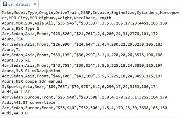
Writing a CSV file

In order to write a comma delimited file we can use the dlm option with a value "csv". The following code writes the file car_data.csv.

proc export data = sashelp.cars
   outfile = '/folders/myfolders/sasuser.v94/TutorialsPoint/car_data.csv'
   dbms = csv;
   run;

On executing the above code we get the below output.

Writing a tab delimited file

In order to write a tab delimited file we can use the dlm option with a value "tab". The following code writes the file car_tab.txt.

proc export data = sashelp.cars
   outfile = '/folders/myfolders/sasuser.v94/TutorialsPoint/car_tab.txt'
   dbms = csv;
   run;

Data can also be written as HTML file which we will see under the output delivery system chapter.

SAS - Concatenate Data Sets

Multiple SAS data sets can be concatenated to give a single data set using the SET statement. The total number of observations in the concatenated data set is the sum of the number of observations in the original data sets. The order of observations is sequential. All observations from the first data set are followed by all observations from the second data set, and so on.

Ideally all the combining data sets have same variables, but in case they have different number of variables, then in the result all the variables appear, with missing values for the smaller data set.

Syntax

The basic syntax for SET statement in SAS is −

SET data-set 1 data-set 2 data-set 3.....;

Following is the description of the parameters used −

data-set1,data-set2 are dataset names written one after another.

Example

Consider the employee data of an organization which is available in two different data sets, one for the IT department and another for Non-It department. To get the complete details of all the employees we concatenate both the data sets using the SET statement shown as below.

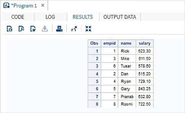
DATA ITDEPT; 
   INPUT empid name $ salary  ; 
DATALINES; 
1 Rick 623.3 
3 Mike 611.5 
6 Tusar 578.6 
; 
RUN; 
DATA NON_ITDEPT; 
   INPUT empid name $ salary  ; 
DATALINES; 
2 Dan 515.2 
4 Ryan 729.1 
5 Gary 843.25 
7 Pranab 632.8 
8 Rasmi 722.5 
RUN; 
DATA All_Dept; 
   SET ITDEPT NON_ITDEPT; 
RUN; 
PROC PRINT DATA = All_Dept; 
RUN;

When the above code is executed, we get the following output.

Scenarios

When we have many variations in the data sets for concatenation, the result of variables can differ but the total number of observations in the concatenated data set is always the sum of the observations in each data set. We will consider below many scenarios on this variation.

Different number of variables

If one of the original data set has more number of variables then another, then the data sets still get combined but in the smaller data set those variables appear as missing.

Example

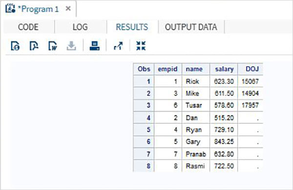
In below example the first data set has an extra variable named DOJ. In the result the value of DOJ for second data set will appear as missing.

DATA ITDEPT; 
   INPUT empid name $ salary DOJ date9.  ; 
DATALINES; 
1 Rick 623.3 02APR2001
3 Mike 611.5 21OCT2000
6 Tusar 578.6 01MAR2009  
; 
RUN; 
DATA NON_ITDEPT; 
   INPUT empid name $ salary  ; 
DATALINES; 
2 Dan 515.2 
4 Ryan 729.1 
5 Gary 843.25 
7 Pranab 632.8 
8 Rasmi 722.5 
RUN; 
DATA All_Dept; 
   SET ITDEPT NON_ITDEPT; 
RUN; 
PROC PRINT DATA = All_Dept; 
RUN;

When the above code is executed, we get the following output.

Different variable name

In this scenario the data sets have same number of variables but a variable name differs between them. In that case a normal concatenation will produce all the variables in the result set and giving missing results for the two variables which differ. While we may not change the variable name in the original data sets we can apply the RENAME function in the concatenated data set we create. That will produce the same result as a normal concatenation but of course with one new variable name in place of two different variable names present in the original data set.

Example

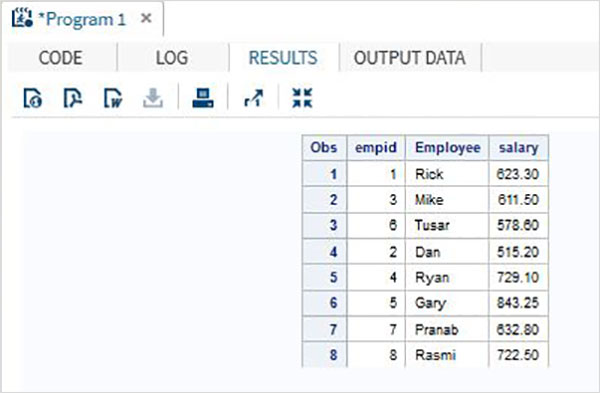
In the below example data set ITDEPT has the variable name ename whereas the data set NON_ITDEPT has the variable name empname. But both of these variables represent the same type(character). We apply the RENAME function in the SET statement as shown below.

DATA ITDEPT; 
   INPUT empid ename $ salary  ; 
DATALINES; 
1 Rick 623.3 
3 Mike 611.5 
6 Tusar 578.6 
; 
RUN; 
DATA NON_ITDEPT; 
   INPUT empid empname $ salary  ; 
DATALINES; 
2 Dan 515.2 
4 Ryan 729.1 
5 Gary 843.25 
7 Pranab 632.8 
8 Rasmi 722.5 
RUN; 
DATA All_Dept; 
   SET ITDEPT(RENAME =(ename = Employee) ) NON_ITDEPT(RENAME =(empname = Employee) ); 
RUN; 
PROC PRINT DATA = All_Dept; 
RUN;

When the above code is executed, we get the following output.

Different variable lengths

If the variable lengths in the two data sets is different than the concatenated data set will have values in which some data is truncated for the variable with smaller length. It happens if the first data set has a smaller length. To solve this we apply the higher length to both the data set as shown below.

Example

In the below example the variable ename is of length 5 in the first data set and 7 in the second. When concatenating we apply the LENGTH statement in the concatenated data set to set the ename length to 7.

DATA ITDEPT; 
   INPUT  empid 1-2 ename $ 3-7 salary 8-14  ; 
DATALINES; 
1 Rick  623.3 
3 Mike  611.5 
6 Tusar 578.6 
; 
RUN;
DATA NON_ITDEPT; 
   INPUT  empid 1-2 ename $ 3-9  salary 10-16 ; 
DATALINES; 
2 Dan    515.2 
4 Ryan   729.1 
5 Gary   843.25
7 Pranab 632.8 
8 Rasmi  722.5 
RUN; 
DATA All_Dept; 
   LENGTH ename $ 7   ;
   SET ITDEPT  NON_ITDEPT ; 
RUN; 
PROC PRINT DATA = All_Dept; 
RUN;

When the above code is executed, we get the following output.

SAS - Merge Data Sets

Multiple SAS data sets can be merged based on a specific common variable to give a single data set. This is done using the MERGE statement and BY statement. The total number of observations in the merged data set is often less than the sum of the number of observations in the original data sets. It is because the variables form both data sets get merged as one record based when there is a match in the value of the common variable.

There are two Prerequisites for merging data sets given below −

input data sets must have at least one common variable to merge on.
input data sets must be sorted by the common variable(s) that will be used to merge on.

Syntax

The basic syntax for MERGE and BY statement in SAS is −

MERGE Data-Set 1 Data-Set 2
BY Common Variable

Following is the description of the parameters used −

Data-set1,Data-set2 are data set names written one after another.
Common Variable is the variable based on whose matching values the data sets will be merged.

Data Merging

Let us understand data merging with the help of an example.

Example

Consider two SAS data sets one containing the employee ID with name and salary and another containing employee ID with employee ID and department. In this case to get the complete information for each employee we can merge these two data sets. The final data set will still have one observation per employee but it will contain both the salary and department variables.

# Data set 1	
ID NAME SALARY	
1 Rick 623.3		 
2 Dan 515.2 		
3 Mike 611.5 		
4 Ryan 729.1 
5 Gary 843.25 
6 Tusar 578.6 
7 Pranab 632.8 
8 Rasmi 722.5 

# Data set 2
ID DEPT
1 IT 
2 OPS
3 IT 
4 HR 
5 FIN 
6 IT 
7 OPS
8 FIN 

# Merged data set
ID NAME SALARY DEPT	
1 Rick 623.3	IT 		 
2 Dan 515.2 	OPS	
3 Mike 611.5 	IT 	
4 Ryan 729.1    HR 
5 Gary 843.25   FIN 
6 Tusar 578.6   IT 
7 Pranab 632.8  OPS
8 Rasmi 722.5   FIN

The above result is achieved by using the following code in which the common variable (ID) is used in the BY statement. Please note that the observations in both the datasets are already sorted in ID column.

DATA SALARY; 
   INPUT empid name $ salary  ; 
DATALINES; 
1 Rick 623.3		 
2 Dan 515.2 		
3 Mike 611.5 		
4 Ryan 729.1 
5 Gary 843.25 
6 Tusar 578.6 
7 Pranab 632.8 
8 Rasmi 722.5 
;
RUN; 
DATA DEPT; 
   INPUT empid dEPT $ ; 
DATALINES; 
1 IT 
2 OPS
3 IT 
4 HR 
5 FIN 
6 IT 
7 OPS
8 FIN 
;
RUN; 
DATA All_details;
MERGE SALARY DEPT;
BY (empid);
RUN;
PROC PRINT DATA = All_details; 
RUN;

Missing Values in the Matching Column

There may be cases when some values of the common variable will not match between the data sets. In such cases the data sets still get merged but give missing values in the result.

Example

Consider the case of employee ID 3 missing from the dataset salary and employee ID 6 missing form data set DEPT. When the above code is applied, we get the below result.

ID NAME SALARY DEPT	
1 Rick 623.3	IT 		 
2 Dan 515.2 	OPS	
3 .		.		IT
4 Ryan 729.1    HR 
5 Gary 843.25   FIN 
6 Tusar 578.6   .
7 Pranab 632.8  OPS
8 Rasmi 722.5   FIN

Merging only the Matches

To avoid the missing values in the result we can consider keeping only the observations with matched values for the common variable. That is achieved by using the IN statement. The merge statement of the SAS program needs to be changed.

Example

In the below example, the IN= value keeps only the observations where the values from both the data sets SALARY and DEPT match.

DATA All_details;
MERGE SALARY(IN = a) DEPT(IN = b);
BY (empid);
IF a = 1 and b = 1;
RUN;
PROC PRINT DATA = All_details; 
RUN;

Upon execution of the above SAS program with the above changed part, we get the following output.

1 Rick 623.3	IT 		 
2 Dan 515.2 	OPS	
4 Ryan 729.1    HR 
5 Gary 843.25   FIN 
7 Pranab 632.8  OPS
8 Rasmi 722.5   FIN

SAS - Subsetting Data Sets

Subsetting a SAS data set means extracting a part of the data set by selecting a fewer number of variables or fewer number of observations or both. While subsetting of variables is done by using KEEP and DROP statement, the sub setting of observations is done using DELETE statement.

Also the resulting data from the subsetting operation is held in a new data set which can be used for further analysis. Sub setting is mainly used for the purpose of analyzing a part of the data set without using those variables or observations which may not be relevant to the analysis.

Subsetting Variables

In this method we extract only few variables from the entire data set.

Syntax

The basic syntax for sub setting variables in SAS is −

KEEP var1 var2 ... ;
DROP var1 var2 ... ;

Following is the description of the parameters used −

var1 and var2 are the variable names from the data set which needs to be kept or dropped.

Example

Consider the below SAS data set containing the employee details of an organization. If we are interested only in getting the Name and Department values from the data set, then we can use the below code.

DATA Employee; 
   INPUT empid ename $ salary DEPT $ ; 
DATALINES; 
1 Rick 623.3 	IT 		 
2 Dan 515.2 	OPS	
3 Mike 611.5 	IT 	
4 Ryan 729.1    HR 
5 Gary 843.25   FIN 
6 Tusar 578.6   IT 
7 Pranab 632.8  OPS
8 Rasmi 722.5   FIN 
;
RUN;
DATA OnlyDept;
   SET Employee;
   KEEP ename DEPT;
   RUN;
   PROC PRINT DATA = OnlyDept; 
RUN;

When the above code is executed, we get the following output.

The same result can be obtained by dropping the variables that are not required. The below code illustrates this.

DATA Employee; 
   INPUT empid ename $ salary DEPT $ ; 
DATALINES; 
1 Rick 623.3 	IT 		 
2 Dan 515.2 	OPS	
3 Mike 611.5 	IT 	
4 Ryan 729.1    HR 
5 Gary 843.25   FIN 
6 Tusar 578.6   IT 
7 Pranab 632.8  OPS
8 Rasmi 722.5   FIN 
;
RUN;
DATA OnlyDept;
   SET Employee;
   DROP empid salary;
   RUN;
   PROC PRINT DATA = OnlyDept; 
RUN;

Subsetting Observations

In this method we extract only few observations from the entire data set.

Syntax

We use PROC FREQ which keeps track of the observations selected for the new data set.

The syntax for sub setting observations is −

IF Var Condition THEN DELETE ;

Following is the description of the parameters used −

Var is the name of the variable based on whose value the observations will be deleted using the specified condition.

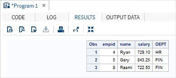
Example

Consider the below SAS data set containing the employee details of an organization. If we are interested only in getting the data for employees with salary greater than 700,then we use the below code.

DATA Employee; 
   INPUT empid name $ salary DEPT $ ; 
DATALINES; 
1 Rick 623.3	IT 		 
2 Dan 515.2 	OPS	
3 Mike 611.5 	IT 	
4 Ryan 729.1    HR 
5 Gary 843.25   FIN 
6 Tusar 578.6   IT 
7 Pranab 632.8  OPS
8 Rasmi 722.5   FIN 
;
RUN;
DATA OnlyDept;
   SET Employee;
   IF salary < 700 THEN DELETE;
   RUN;
   PROC PRINT DATA = OnlyDept; 
RUN;

When the above code is executed, we get the following output.

SAS - Format Data Sets

Sometimes we prefer to show the analyzed data in a format which is different from the format in which it is already present in the data set. For example we want to add the dollar sign and two decimal places to a variable which has price information. Or we may want to show a text variable, all in uppercase. We can use FORMAT to apply the in-built SAS formats and PROC FORMAT is to apply user defined formats. Also a single format can be applied to multiple variables.

Syntax

The basic syntax for applying in-built SAS formats is −

format variable name format name

Following is the description of the parameters used −

variable name is the variable name used in dataset.
format name is the data format to be applied on the variable.

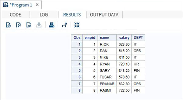
Example

Let's consider the below SAS data set containing the employee details of an organization. We wish to show all the names in uppercase. The formatstatement is used to achieve this.

DATA Employee; 
   INPUT empid name $ salary DEPT $ ; 
   format name $upcase9. ;
DATALINES; 
1 Rick 623.3	IT 		 
2 Dan 515.2 	OPS	
3 Mike 611.5 	IT 	
4 Ryan 729.1    HR 
5 Gary 843.25   FIN 
6 Tusar 578.6   IT 
7 Pranab 632.8  OPS
8 Rasmi 722.5   FIN 
;
RUN;
   PROC PRINT DATA = Employee; 
RUN;

When the above code is executed, we get the following output.

Using PROC FORMAT

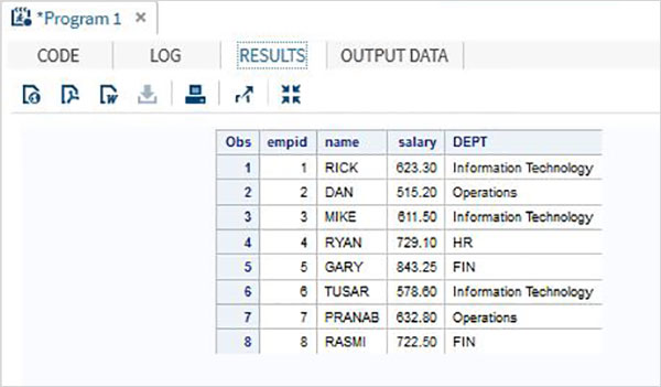
We can also use PROC FORMAT to format data. In the below example we assign new values to the variable DEPT exapnding the name of the department.

DATA Employee; 
   INPUT empid name $ salary DEPT $ ; 

DATALINES; 
1 Rick 623.3 IT 		 
2 Dan 515.2 OPS
3 Mike 611.5 IT 	
4 Ryan 729.1 HR 
5 Gary 843.25 FIN 
6 Tusar 578.6 IT 
7 Pranab 632.8 OPS
8 Rasmi 722.5 FIN 
;
proc format;
value $DEP 'IT' = 'Information Technology'
      'OPS'= 'Operations' ;
RUN;
   PROC PRINT DATA = Employee; 
   format name $upcase9. DEPT $DEP.; 
RUN;

When the above code is executed, we get the following output.

SAS - SQL

SAS offers extensive support to most of the popular relational databases by using SQL queries inside SAS programs. Most of the ANSI SQL syntax is supported. The procedure PROC SQL is used to process the SQL statements. This procedure can not only give back the result of an SQL query, it can also create SAS tables & variables. The example of all these scenarios is described below.

Syntax

The basic syntax for using PROC SQL in SAS is −

PROC SQL;
SELECT Columns
FROM TABLE
WHERE Columns
GROUP BY Columns
;
QUIT;

Following is the description of the parameters used −

the SQL query is written below the PROC SQL statement followed by the QUIT statement.

Below we will see how this SAS procedure can be used for the CRUD (Create, Read, Update and Delete)operations in SQL.

SQL Create Operation

Using SQL we can create new data set form raw data. In the below example, first we declare a data set named TEMP containing the raw data. Then we write a SQL query to create a table from the variables of this data set.

DATA TEMP;
INPUT ID $ NAME $ SALARY DEPARTMENT $;
DATALINES;
1 Rick 623.3 IT
2 Dan 515.2 Operations
3 Michelle 611 IT
4 Ryan 729 HR
5 Gary 843.25 Finance
6 Nina 578 IT
7 Simon 632.8 Operations
8 Guru 722.5 Finance
;
RUN;

PROC SQL;
CREATE TABLE EMPLOYEES AS
SELECT * FROM TEMP;
QUIT;

PROC PRINT data = EMPLOYEES;
RUN;

When the above code is executed we get the following result −

SQL Read Operation

The Read operation in SQL involves writing SQL SELECT queries to read the data from the tables. In The below program queries the SAS data set named CARS available in the library SASHELP. The query fetches some of the columns of the data set.

PROC SQL;
SELECT make,model,type,invoice,horsepower
FROM 
SASHELP.CARS
;
QUIT;

When the above code is executed we get the following result −

SQL SELECT with WHERE Clause

The below program queries the CARS data set with a where clause. In the result we get only the observation which have make as 'Audi' and type as 'Sports'.

PROC SQL;
SELECT make,model,type,invoice,horsepower
FROM 
SASHELP.CARS
Where make = 'Audi'
and Type = 'Sports'
;
QUIT;

When the above code is executed we get the following result −

SQL UPDATE Operation

We can update the SAS table using the SQL Update statement. Below we first create a new table named EMPLOYEES2 and then update it using the SQL UPDATE statement.

DATA TEMP;
INPUT ID $ NAME $ SALARY DEPARTMENT $;
DATALINES;
1 Rick 623.3 IT
2 Dan 515.2 Operations
3 Michelle 611 IT
4 Ryan 729 HR
5 Gary 843.25 Finance
6 Nina 578 IT
7 Simon 632.8 Operations
8 Guru 722.5 Finance
;
RUN;

PROC SQL;
CREATE TABLE EMPLOYEES2 AS
SELECT ID as EMPID,
Name as EMPNAME ,
SALARY as SALARY,
DEPARTMENT as DEPT,
SALARY*0.23 as COMMISION
FROM TEMP;
QUIT;

PROC SQL;
UPDATE EMPLOYEES2
      SET SALARY = SALARY*1.25;
   QUIT;
      PROC PRINT data = EMPLOYEES2;
RUN;

When the above code is executed we get the following result −

SQL DELETE Operation

The delete operation in SQL involves removing certain values from the table using the SQL DELETE statement. We continue to use the data from the above example and delete the rows from the table in which the salary of the employees is greater than 900.

PROC SQL;
DELETE FROM EMPLOYEES2
      WHERE SALARY > 900;
QUIT;
      PROC PRINT data = EMPLOYEES2;
RUN;

When the above code is executed we get the following result −

SAS - ODS

The output from a SAS program can be converted to more user friendly forms like .html or PDF. This is done by using the ODS statement available in SAS. ODS stands for output delivery system. It is mostly used to format the output data of a SAS program to nice reports which are good to look at and understand. That also helps sharing the output with other platforms and soft wares. It can also combine the results from multiple PROC statements in one single file.

Syntax

The basic syntax for using the ODS statement in SAS is −

ODS outputtype
PATH path name
FILE = Filename and Path
STYLE = StyleName
;
PROC some proc
;
ODS outputtype CLOSE;

Following is the description of the parameters used −

PATH represents the statement used in case of HTML output. In other types of output we include the path in the filename.
Style represents one of the in-built styles available in the SAS environment.

Creating HTML Output

We create HTML output using the ODS HTML statement.In the below example we create a html file in our desired path. We apply a style available in the styles library. We can see the output file in the mentioned path and we can download it to save in an environment different from the SAS environment. Please note that we have two proc SQL statements and both their output is captured into a single file.

ODS HTML 
   PATH = '/folders/myfolders/sasuser.v94/TutorialsPoint/'
   FILE = 'CARS2.html'
   STYLE = EGDefault;
proc SQL;
select make, model, invoice 
from sashelp.cars
where make in ('Audi','BMW')
and type = 'Sports'
;
quit;

proc SQL;
select make,mean(horsepower)as meanhp
from sashelp.cars
where make in ('Audi','BMW')
group by make;
quit;

ODS HTML CLOSE;

When the above code is executed we get the following result −

Creating PDF Output

In the below example we create a PDF file in our desired path. We apply a style available in the styles library. We can see the output file in the mentioned path and we can download it to save in an environment different from the SAS environment. Please note that we have two proc SQL statements and both their output is captured into a single file.

ODS PDF 
   FILE = '/folders/myfolders/sasuser.v94/TutorialsPoint/CARS2.pdf'
   STYLE = EGDefault;
proc SQL;
select make, model, invoice 
from sashelp.cars
where make in ('Audi','BMW')
and type = 'Sports'
;
quit;

proc SQL;
select make,mean(horsepower)as meanhp
from sashelp.cars
where make in ('Audi','BMW')
group by make;
quit;

ODS PDF CLOSE;

When the above code is executed we get the following result −

Creating TRF(Word) Output

In the below example we create a RTF file in our desired path. We apply a style available in the styles library. We can see the output file in the mentioned path and we can download it to save in an environment different from the SAS environment. Please note that we have two proc SQL statements and both their output is captured into a single file.

ODS RTF 
FILE = '/folders/myfolders/sasuser.v94/TutorialsPoint/CARS.rtf'
STYLE = EGDefault;
proc SQL;
select make, model, invoice 
from sashelp.cars
where make in ('Audi','BMW')
and type = 'Sports'
;
quit;

proc SQL;
select make,mean(horsepower)as meanhp
from sashelp.cars
where make in ('Audi','BMW')
group by make;
quit;

ODS rtf CLOSE;

When the above code is executed we get the following result −

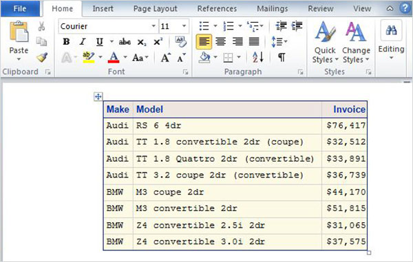
SAS - Simulations

Simulation is a computational technique that uses repeating computation on many different random samples in order to estimate a statistical quantity. Using SAS we can simulate complex data that have specified statistical properties in real-world system. We use software to build a model of the system and numerically generate data that you can be used for a better understanding of the behavior of the real-world system. Part of the art of designing a computer simulation model is deciding which aspects of the real-life system are necessary to include in the model so that the data generated by the model can be used to make effective decisions. Because of this complexity, SAS has a dedicated software component for Simulation.

The SAS software component which is used in creating SAS simulation is called SAS Simulation Studio. Its graphical user interface provides a full set of tools for building, executing, and analyzing the results of discrete event simulation models.

Different types of statistical distributions on which SAS simulation can be applied is listed below.

SIMULATE DATA FROM A CONTINUOUS DISTRIBUTION
SIMULATE DATA FROM A DISCRETE DISTRIBUTION
SIMULATE DATA FROM A MIXTURE OF DISTRIBUTIONS
SIMULATE DATA FROM A COMPLEX DISTRIBUTION
SIMULATE DATA FROM A MULTIVARIATE DISTRIBUTION
APPROXIMATE A SAMPLING DISTRIBUTION
ASSESS REGRESSION ESTIMATES

SAS - Histograms

A Histogram is graphical display of data using bars of different heights. It groups the various numbers in the data set into many ranges. It also represents the estimation of the probability of distribution of a continuous variable. In SAS the PROC UNIVARIATE is used to create histograms with the below options.

Syntax

The basic syntax to create a histogram in SAS is −

PROC UNIVARAITE DATA = DATASET;
HISTOGRAM variables;
RUN;

Following is the description of parameters used −

DATASET is the name of the dataset used.
variables are the values used to plot the histogram.

Simple Histogram

A simple histogram is created by specifying the name of the variable and the range to be considered to group the values.

Example

In the below example, we consider the minimum and maximum values of the variable horsepower and take a range of 50. So the values form a group in steps of 50.

proc univariate data = sashelp.cars;
   histogram horsepower
   / midpoints = 176 to 350 by 50;
run;

When we execute the above code, we get the following output −

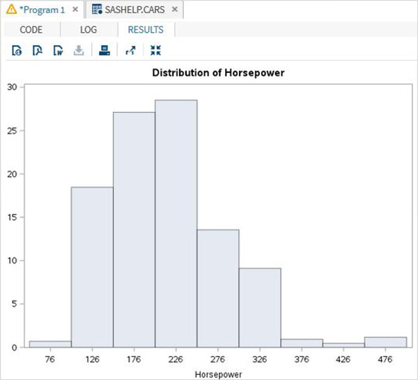
Histogram with Curve Fitting

We can fit some distribution curves into the histogram using additional options.

Example

In the below example we fit a distribution curve with mean and standard deviation values mentioned as EST. This option uses and estimate of the parameters.

proc univariate data = sashelp.cars noprint;
histogram horsepower
/ 
normal ( 
   mu = est
   sigma = est
   color = blue
   w = 2.5 
)
barlabel = percent
midpoints = 70 to 550 by 50;
run;

When we execute the above code, we get the following output −

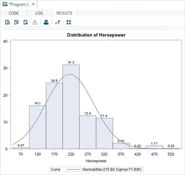
SAS - Bar Charts

A bar chart represents data in rectangular bars with length of the bar proportional to the value of the variable. SAS uses the procedure PROC SGPLOT to create bar charts. We can draw both simple and stacked bars in the bar chart. In bar chart each of the bars can be given different colors.

Syntax

The basic syntax to create a bar-chart in SAS is −

PROC SGPLOT DATA = DATASET;
VBAR variables;
RUN;

Following is the description of parameters used −

DATASET − is the name of the dataset used.
variables − are the values used to plot the histogram.

Simple Bar chart

A simple bar chart is a bar chart in which a variable from the dataset is represented as bars.

Example

The below script will create a bar-chart representing the length of cars as bars.

PROC SQL;
create table CARS1 as
SELECT make, model, type, invoice, horsepower, length, weight
   FROM 
   SASHELP.CARS
   WHERE make in ('Audi','BMW')
;
RUN;

proc SGPLOT data = work.cars1;
vbar length ;
title 'Lengths of cars';
run;
quit;

When we execute the above code, we get the following output −

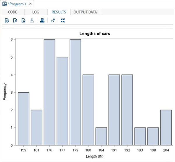
Stacked Bar chart

A stacked bar chart is a bar chart in which a variable from the dataset is calculated with respect to another variable.

Example

The below script will create a stacked bar-chart where the length of the cars are calculated for each car type. We use the group option to specify the second variable.

proc SGPLOT data = work.cars1;
vbar length /group = type ;
title 'Lengths of Cars by Types';
run;
quit;

When we execute the above code, we get the following output −

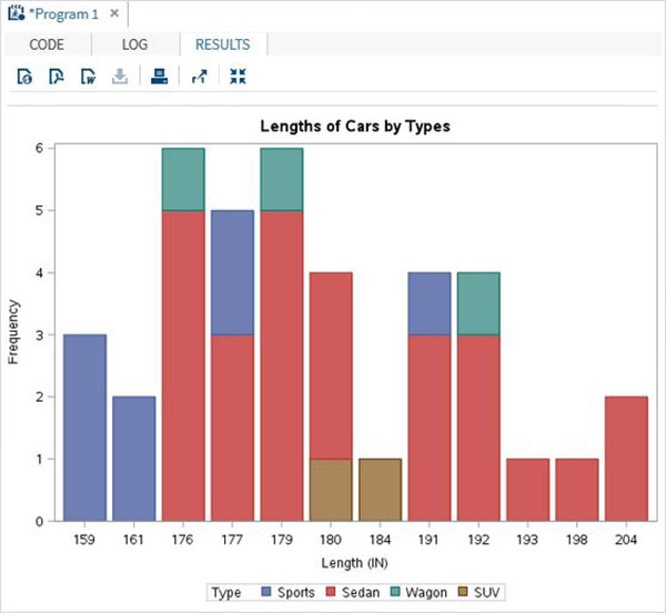
Clustered Bar chart

The clustered bar chart is created to show how the values of a variable are spread across a culture.

Example

The below script will create a clustered bar-chart where the length of the cars is clustered around the car type.So we see two adjacent bars at length 191, one for the car type 'Sedan' and another for the car type 'Wagon'.

proc SGPLOT data = work.cars1;
vbar length /group = type GROUPDISPLAY = CLUSTER;
title 'Cluster of Cars by Types';
run;
quit;

When we execute the above code, we get the following output −

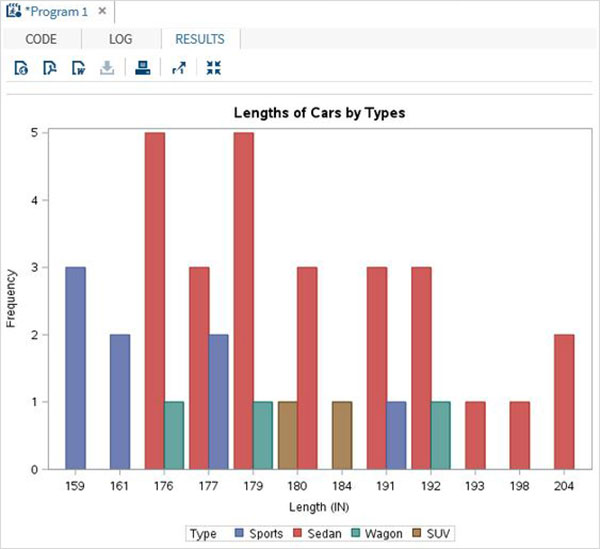
SAS - Pie Charts

A pie-chart is a representation of values as slices of a circle with different colors. The slices are labeled and the numbers corresponding to each slice is also represented in the chart.

In SAS the pie chart is created using PROC TEMPLATE which takes parameters to control percentage, labels, color, title etc.

Syntax

The basic syntax to create a pie-chart in SAS is −

PROC TEMPLATE;
   DEFINE STATGRAPH pie;
      BEGINGRAPH;
         LAYOUT REGION;
            PIECHART CATEGORY = variable /
            DATALABELLOCATION = OUTSIDE
            CATEGORYDIRECTION = CLOCKWISE
            START = 180 NAME = 'pie';
            DISCRETELEGEND 'pie' /
            TITLE = ' ';
         ENDLAYOUT;
      ENDGRAPH;
   END;
RUN;

Following is the description of parameters used −

variable is the value for which we create the pie chart.

Simple Pie Chart

In this pie chart we take a single variable form the dataset. The pie chart is created with value of the slices representing the fraction of the count of the variable with respect to the total value of the variable.

Example

In the below example each slice represents the fraction of the type of car from the total number of cars.

PROC SQL;
create table CARS1 as
SELECT make, model, type, invoice, horsepower, length, weight
 FROM 
SASHELP.CARS
WHERE make in ('Audi','BMW')
;
RUN;

PROC TEMPLATE;
   DEFINE STATGRAPH pie;
      BEGINGRAPH;
         LAYOUT REGION;
            PIECHART CATEGORY = type /
            DATALABELLOCATION = OUTSIDE
            CATEGORYDIRECTION = CLOCKWISE
            START = 180 NAME = 'pie';
            DISCRETELEGEND 'pie' /
            TITLE = 'Car Types';
         ENDLAYOUT;
      ENDGRAPH;
   END;
RUN;
PROC SGRENDER DATA = cars1
            TEMPLATE = pie;
RUN;

When we execute the above code, we get the following output −

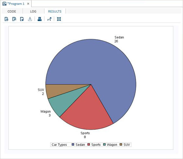
Pie Chart with Data Labels

In this pie chart we represent both the fractional value as well as the percentage value for each slice. We also change the location of the label to be inside the chart. The style of appearance of the chart is modified by using the DATASKIN option. It uses one of the inbuilt styles, available in the SAS environment.

Example

PROC TEMPLATE;
   DEFINE STATGRAPH pie;
      BEGINGRAPH;
         LAYOUT REGION;
            PIECHART CATEGORY = type /
            DATALABELLOCATION = INSIDE
            DATALABELCONTENT = ALL
            CATEGORYDIRECTION = CLOCKWISE
            DATASKIN = SHEEN 
            START = 180 NAME = 'pie';
            DISCRETELEGEND 'pie' /
            TITLE = 'Car Types';
         ENDLAYOUT;
      ENDGRAPH;
   END;
RUN;
PROC SGRENDER DATA = cars1
            TEMPLATE = pie;
RUN;

When we execute the above code, we get the following output −

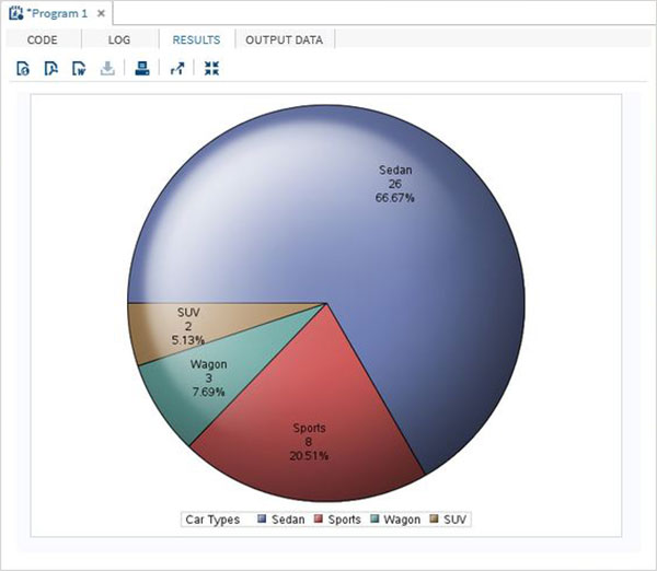
Grouped Pie Chart

In this pie chart the value of the variable presented in the graph is grouped with respect to another variable of the same data set. Each group becomes one circle and the chart has as many concentric circles as the number of groups available.

Example

In the below example we group the chart with respect to the variable named "Make". As there are two values available ("Audi" and "BMW") so we get two concentric circles each representing slices of car types in its own make.

PROC TEMPLATE;
   DEFINE STATGRAPH pie;
      BEGINGRAPH;
         LAYOUT REGION;
            PIECHART CATEGORY = type / Group = make
            DATALABELLOCATION = INSIDE
            DATALABELCONTENT = ALL
            CATEGORYDIRECTION = CLOCKWISE
            DATASKIN = SHEEN 
            START = 180 NAME = 'pie';
            DISCRETELEGEND 'pie' /
            TITLE = 'Car Types';
         ENDLAYOUT;
      ENDGRAPH;
   END;
RUN;
PROC SGRENDER DATA = cars1
            TEMPLATE = pie;
RUN;

When we execute the above code, we get the following output −

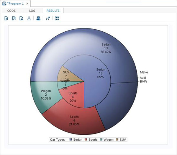
SAS - Scatter Plots

A scatterplot is a type of graph which uses values from two variables plotted in a Cartesian plane. It is usually used to find out the relationship between two variables. In SAS we use PROC SGSCATTER to create scatterplots.

Please note that we create the data set named CARS1 in the first example and use the same data set for all the subsequent data sets. This data set remains in the work library till the end of the SAS session.

Syntax

The basic syntax to create a scatter-plot in SAS is −

PROC sgscatter  DATA = DATASET;
   PLOT VARIABLE_1 * VARIABLE_2
   / datalabel = VARIABLE group = VARIABLE;
RUN;

Following is the description of parameters used −

DATASET is the name of data set.
VARIABLE is the variable used from the dataset.

Simple Scatterplot

In a simple scatterplot we choose two variables form the dataset and group them with respect a third variable. We can also label the data. The result shows how the two variables are scattered in the Cartesian plane.

Example

PROC SQL;
create table CARS1 as
SELECT make, model, type, invoice, horsepower, length, weight
FROM 
SASHELP.CARS
WHERE make in ('Audi','BMW')
;
RUN;

TITLE 'Scatterplot - Two Variables';
PROC sgscatter  DATA = CARS1;
   PLOT horsepower*Invoice 
   / datalabel = make group = type grid;
   title 'Horsepower vs. Invoice for car makers by types';
RUN;

When we execute the above code, we get the following output −

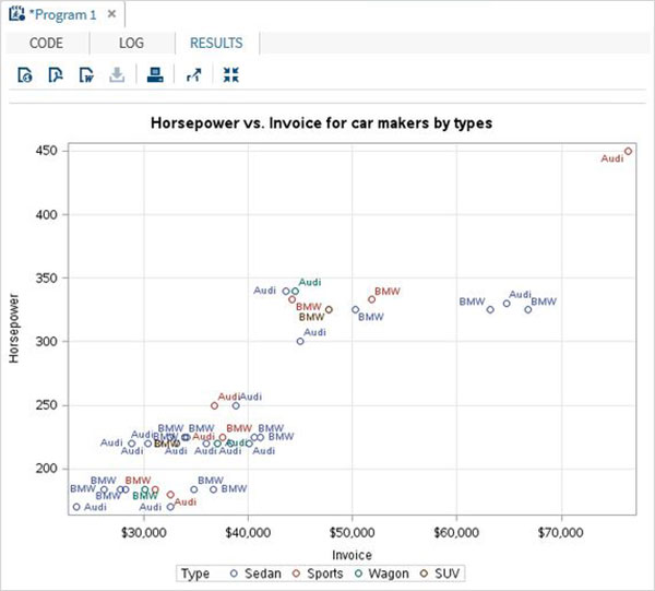
Scatterplot with Prediction

we can use an estimation parameter to predict the strength of correlation between by drawing an ellipse around the values. We use the additional options in the procedure to draw the ellipse as shown below.

Example

proc sgscatter data = cars1; 
compare y = Invoice  x = (horsepower length)  
         / group = type  ellipse =(alpha = 0.05 type = predicted); 
title
'Average Invoice vs. horsepower for cars by length'; 
title2
'-- with 95% prediction ellipse --'
; 
format
Invoice dollar6.0;
run;

When we execute the above code, we get the following output −

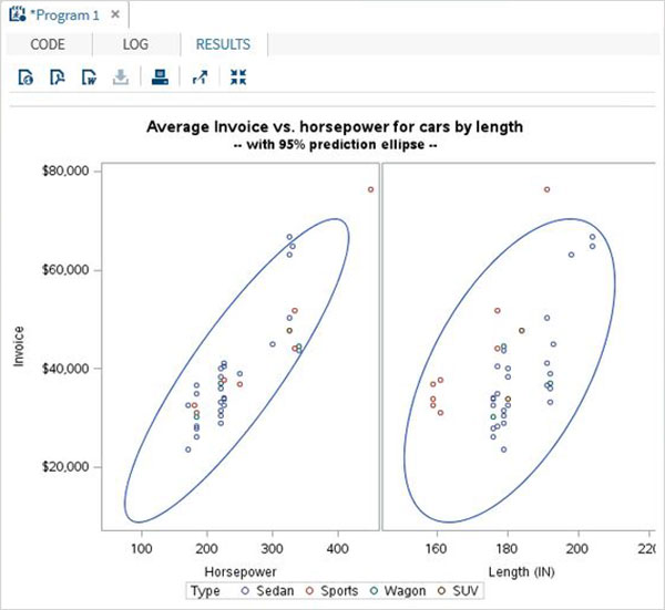
Scatter Matrix

We can also have a scatterplot involving more than two variables by grouping them into pairs. In the example below we consider three variables and draw a scatter plot matrix. We get 3 pairs of resulting matrix.

Example

PROC sgscatter  DATA = CARS1;
   matrix horsepower invoice length
   / group = type;

   title 'Horsepower vs. Invoice vs. Length for car makers by types';
RUN;

When we execute the above code, we get the following output −

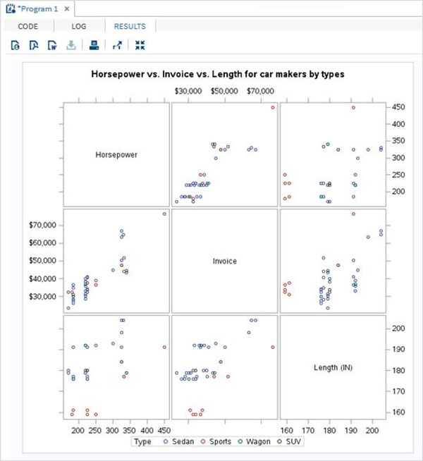
SAS - Box Plots

A Boxplot is graphical representation of groups of numerical data through their quartiles. Box plots may also have lines extending vertically from the boxes (whiskers) indicating variability outside the upper and lower quartiles. The bottom and top of the box are always the first and third quartiles, and the band inside the box is always the second quartile (the median). In SAS a simple Boxplot is created using PROC SGPLOT and paneled boxplot is created using PROC SGPANEL.

Syntax

The basic syntax to create a boxplot in SAS is −

PROC SGPLOT  DATA = DATASET;
   VBOX VARIABLE / category = VARIABLE;
RUN; 

PROC SGPANEL  DATA = DATASET;;
PANELBY VARIABLE;
   VBOX VARIABLE> / category = VARIABLE;
RUN;

Following is the description of parameters used −

DATASET − is the name of the dataset used.
VARIABLE − is the value used to plot the Boxplot.

Simple Boxplot

In a simple Boxplot we choose one variable from the data set and another to form a category. The values of the first variable are categorized in as many number of groups as the number of distinct values in the second variable.

Example

In the below example we choose the variable horsepower as the first variable and type as the category variable. So we get boxplots for the distribution of values of horsepower for each type of car.

PROC SQL;
create table CARS1 as
SELECT make, model, type, invoice, horsepower, length, weight
   FROM 
   SASHELP.CARS
   WHERE make in ('Audi','BMW')
;
RUN;

PROC SGPLOT  DATA = CARS1;
   VBOX horsepower 
   / category = type;

   title 'Horsepower of cars by types';
RUN;

When we execute the above code, we get the following output −

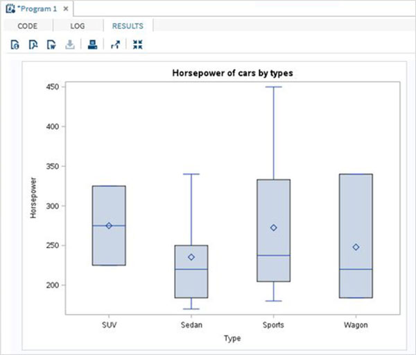
Boxplot in Vertical Panels

We can divide the Boxplots of a variable into many vertical panels(columns). Each panel holds the boxplots for all the categorical variables. But the boxplots are further grouped using another third variable which divides the graph into multiple panels.

Example

In the below example we have paneled the graph using the variable 'make'. As there are two distinct values of 'make' so we get two vertical panels.

PROC SGPANEL  DATA = CARS1;
PANELBY MAKE;
   VBOX horsepower   / category = type;

   title 'Horsepower of cars by types';
RUN;

When we execute the above code, we get the following output −

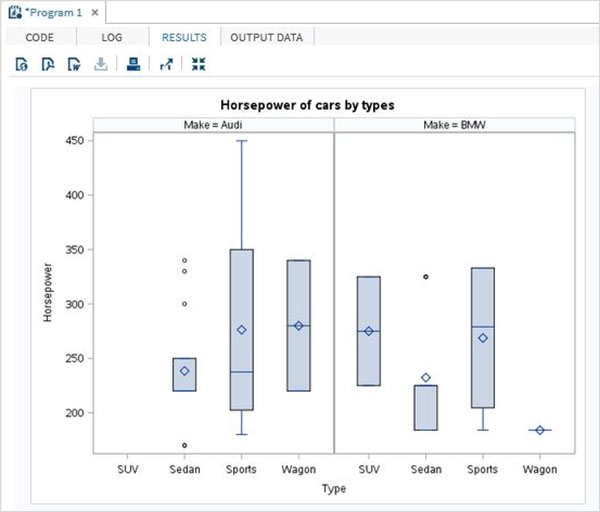
Boxplot in Horizontal Panels

We can divide the Boxplots of a variable into many horizontal panels(rows). Each panel holds the boxplots for all the categorical variables. But the boxplots are further grouped using another third variable which divides the graph into multiple panels. In the below example we have paneled the graph using the variable 'make'. As there are two distinct values of 'make' so we get two horizontal panels.

PROC SGPANEL  DATA = CARS1;
PANELBY MAKE / columns = 1 novarname;

   VBOX horsepower   / category = type;

   title 'Horsepower of cars by types';
RUN;

When we execute the above code, we get the following output −

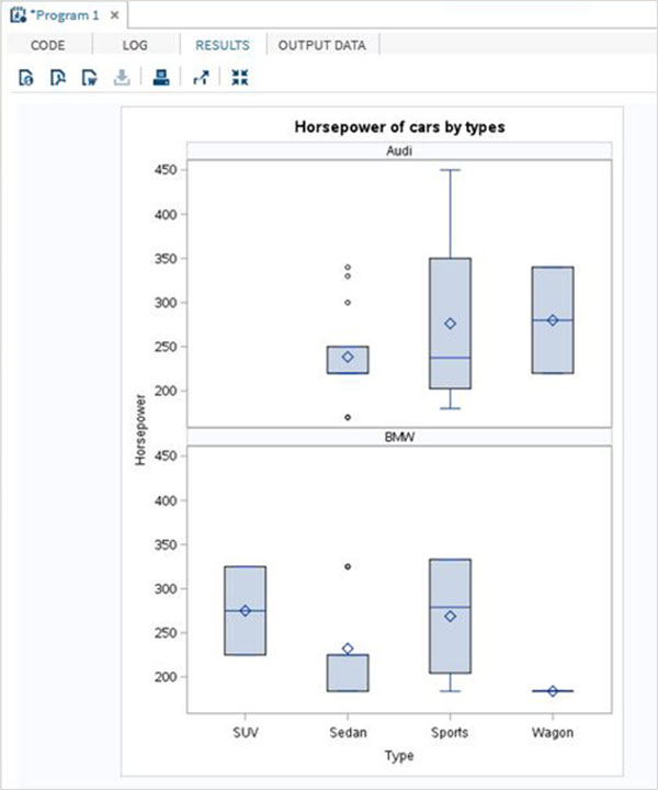
SAS - Arithmetic Mean

The arithmetic mean is the value obtained by summing value of numeric variables and then dividing the sum with the number of variables. It is also called Average. In SAS arithmetic mean is calculated using PROC MEANS. Using this SAS procedure we can find the mean of all variables or some variables of a dataset. We can also form groups and find mean of variables of values specific to that group.

Syntax

The basic syntax for calculating arithmetic mean in SAS is −

PROC MEANS DATA = DATASET;
CLASS Variables ;
VAR Variables;

Following is the description of parameters used −

DATASET − is the name of the dataset used.
Variables − are the name of the variable from the dataset.

Mean of a Dataset

The mean of each of the numeric variable in a dataset is calculated by using the PROC by supplying only the dataset name without any variables.

Example

In the below example we find the mean of all the numeric variables in the SAS dataset named CARS. We specify the maximum digits after decimal place to be 2 and also find the sum of those variables.

PROC MEANS DATA = sashelp.CARS Mean SUM MAXDEC=2;
RUN;

When the above code is executed, we get the following output −

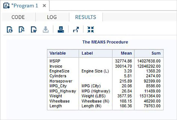
Mean of Select Variables

We can get the mean of some of the variables by supplying their names in the var option.

Example

In the below we calculate the mean of three variables.

PROC MEANS DATA = sashelp.CARS mean SUM MAXDEC=2 ;
var horsepower invoice EngineSize;
RUN;

When the above code is executed, we get the following output −

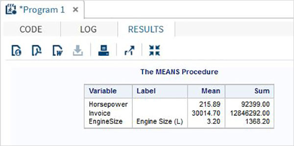
Mean by Class

We can find the mean of the numeric variables by organizing them to groups by using some other variables.

Example

In the example below we find the mean of the variable horsepower for each type under each make of the car.

PROC MEANS DATA = sashelp.CARS mean SUM MAXDEC=2;
class make type;
var horsepower;
RUN;

When the above code is executed, we get the following output −

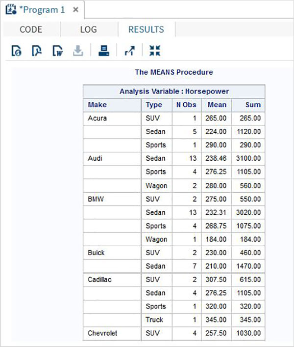
SAS - Standard Deviation

Standard deviation (SD) is a measure of how varied is the data in a data set. Mathematically it measures how distant or close are each value to the mean value of a data set. A standard deviation value close to 0 indicates that the data points tend to be very close to the mean of the data set and a high standard deviation indicates that the data points are spread out over a wider range of values

In SAS the SD values is measured using PROC MEAN as well as PROC SURVEYMEANS.

Using PROC MEANS

To measure the SD using proc means we choose the STD option in the PROC step. It brings out the SD values for each numeric variable present in the data set.

Syntax

The basic syntax for calculating standard deviation in SAS is −

PROC means DATA = dataset STD;

Following is the description of the parameters used −

Dataset − is the name of the dataset.

Example

In the below example we create the data set CARS1 form the CARS data set in the SASHELP library. We choose the STD option with the PROC means step.

PROC SQL;
create table CARS1 as
SELECT make, type, invoice, horsepower, length, weight
   FROM 
   SASHELP.CARS
   WHERE make in ('Audi','BMW')
;
RUN;

proc means data = CARS1 STD;
run;

When we execute the above code it gives the following output −

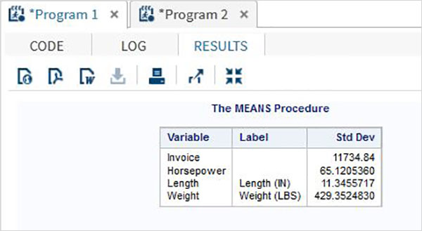
Using PROC SURVEYMEANS

This procedure is also used for measurement of SD along with some advance features like measuring SD for categorical variables as well as provide estimates in variance.

Syntax

The syntax for using PROC SURVEYMEANS is −

PROC SURVEYMEANS options statistic-keywords ;
BY variables ;
CLASS variables ;
VAR variables ;

Following is the description of the parameters used −

BY − indicates the variables used to create groups of observations.
CLASS − indicates the variables used for categorical variables.
VAR − indicates the variables for which SD will be calculated.

Example

The below example describes the use of class option which creates the statistics for each of the values in the class variable.

proc surveymeans data = CARS1 STD;
class type;
var type horsepower;
ods output statistics = rectangle;
run;
proc print data = rectangle;
run;

When we execute the above code it gives the following output −

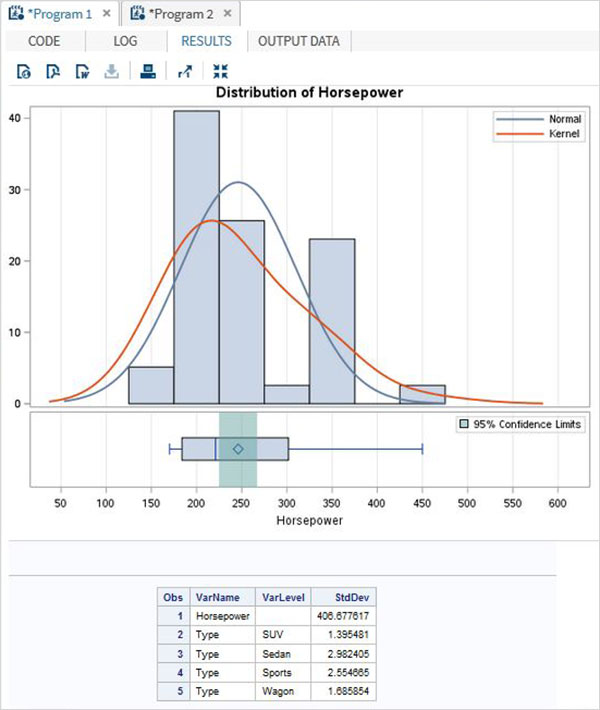
Using BY option

The below code gives example of BY option. In it the result is grouped for each value in the BY option.

Example

proc surveymeans data = CARS1 STD;
var horsepower;
BY make;
ods output statistics = rectangle;
run;
proc print data = rectangle;
run;

When we execute the above code it gives the following output −

Result for make = "Audi"

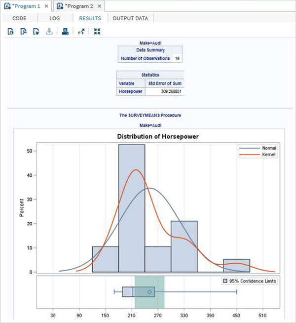
Result for make = "BMW"

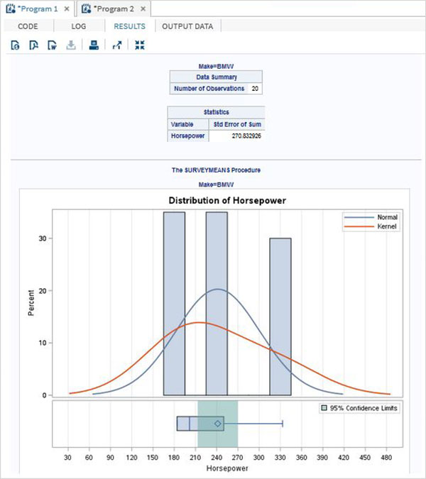
SAS - Frequency Distributions

A frequency distribution is a table showing the frequency of the data points in a data set. Each entry in the table contains the frequency or count of the occurrences of values within a particular group or interval, and in this way, the table summarizes the distribution of values in the sample.

SAS provides a procedure called PROC FREQ to calculate the frequency distribution of data points in a data set.

Syntax

The basic syntax for calculating frequency distribution in SAS is −

PROC FREQ DATA = Dataset ;
TABLES Variable_1 ;
BY Variable_2 ;

Following is the description of the parameters used −

Dataset is the name of the dataset.
Variables_1 is the variable names of the dataset whose frequency distribution needs to be calculated.
Variables_2 is the variables which categorised the frequency distribution result.

Single Variable Frequency Distribution

We can determine the frequency distribution of a single variable by using PROC FREQ. In this case the result will show the frequency of each value of the variable. The result also shows the percentage distribution, cumulative frequency and cumulative percentage.

Example

In the below example we find the frequency distribution of the variable horsepower for the dataset named CARS1 which is created form the library SASHELP.CARS. We can see the result divided into two categories of results. One for each make of the car.

PROC SQL;
create table CARS1 as
SELECT make, model, type, invoice, horsepower, length, weight
   FROM 
   SASHELP.CARS
   WHERE make in ('Audi','BMW')
;
RUN;

proc FREQ data = CARS1 ;
tables horsepower; 
by make;
run;

When the above code is executed, we get the following result −

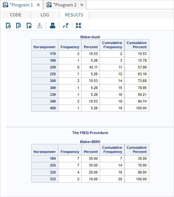
Multiple Variable Frequency Distribution

We can find the frequency distributions for multiple variables which groups them into all possible combinations.

Example

In the below example we calculate the frequency distribution for the make of a car for grouped by car type and also the frequency distribution of each type of car grouped by each make.

proc FREQ data = CARS1 ;
tables make type; 
run;

When the above code is executed, we get the following result −

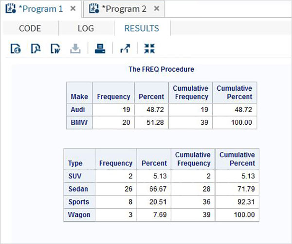
Frequency Distribution with Weight

With the weight option we can calculate the frequency distribution biased with the weight of the variable. Here the value of the variable is taken as the number of observations instead of the count of value.

Example

In the below example we calculate the frequency distribution of the variables make and type with weight assigned to horsepower.

proc FREQ data = CARS1 ;
tables make type; 
weight horsepower;
run;

When the above code is executed, we get the following result −

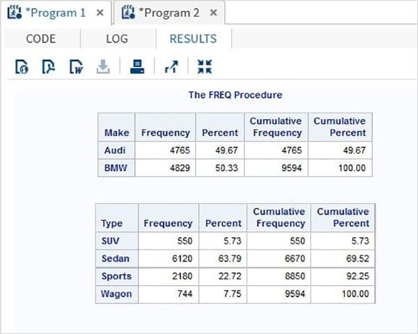
SAS - Cross Tabulations

Cross tabulation involves producing cross tables also called contingent tables using all possible combinations of two or more variables. In SAS it is created using PROC FREQ along with the TABLES option. For example - if we need the frequency of each model for each make in each car type category, then we need to use the TABLES option of PROC FREQ.

Syntax

The basic syntax for applying cross tabulation in SAS is −

PROC FREQ DATA = dataset;
TABLES variable_1*Variable_2;

Following is the description of the parameters used −

Dataset is the name of the dataset.
Variable_1 and Variable_2 are the variable names of the dataset whose frequency distribution needs to be calculated.

Example

Consider the case of finding how many car types are available under each car brand from the dataset cars1 which is created form SASHELP.CARS as shown below. In this case we need the individual frequency values as well as the sum of the frequency values across the makes and across the types. We can observer that the result shows values across the rows and the columns.

PROC SQL;
create table CARS1 as
SELECT make, type, invoice, horsepower, length, weight
   FROM 
   SASHELP.CARS
   WHERE make in ('Audi','BMW')
;
RUN;

proc FREQ data = CARS1;
tables make*type; 
run;

When the above code is executed, we get the following result −

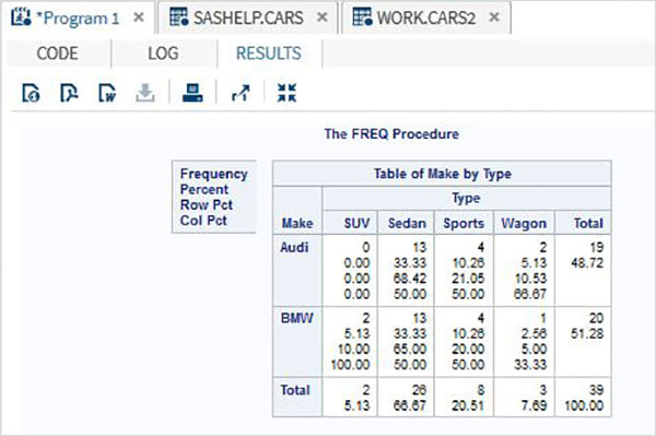
Cross tabulation of 3 Variables

When we have three variables we can group 2 of them and cross tabulate each of these two with the third varaible. So in the result we have two cross tables.

Example

In the below example we find the frequency of each type of car and each model of car with respect to the make of the car. Also we use the nocol and norow option to avoid the sum and percentage values.

proc FREQ data = CARS2 ;
tables make * (type model)  / nocol norow nopercent;   
run;

When the above code is executed, we get the following result −

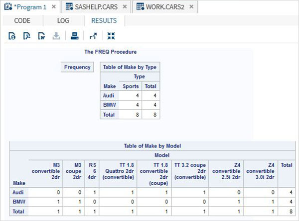
Cross tabulation of 4 Variables

With 4 variables, the number of paired combinations increases to 4. Each variable from group 1 is paired with each variable of group 2.

Example

In the below example we find the frequency of length of the car for each make and each model. Similarly the frequency of horsepower for each make and each model.

proc FREQ data = CARS2 ;
tables (make model) * (length  horsepower)  / nocol norow nopercent;   
run;

When the above code is executed, we get the following result −

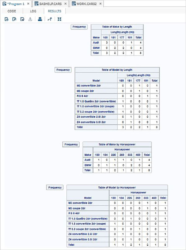
SAS - T Tests

The T-tests are performed to compute the confidence limits for one sample or two independent samples by comparing their means and mean differences. The SAS procedure named PROC TTEST is used to carry out t tests on a single variable and pair of variables.

Syntax

The basic syntax for applying PROC TTEST in SAS is −

PROC TTEST DATA = dataset;
VAR variable;
CLASS Variable;
PAIRED Variable_1 * Variable_2;

Following is the description of the parameters used −

Dataset is the name of the dataset.
Variable_1 and Variable_2 are the variable names of the dataset used in t test.

Example

Below we see one sample t test in which find the t test estimation for the variable horsepower with 95 percent confidence limits.

PROC SQL;
create table CARS1 as
SELECT make, type, invoice, horsepower, length, weight
   FROM 
   SASHELP.CARS
   WHERE make in ('Audi','BMW')
;
RUN;

proc ttest data = cars1 alpha = 0.05 h0 = 0;
 	var horsepower;
   run;

When the above code is executed, we get the following result −

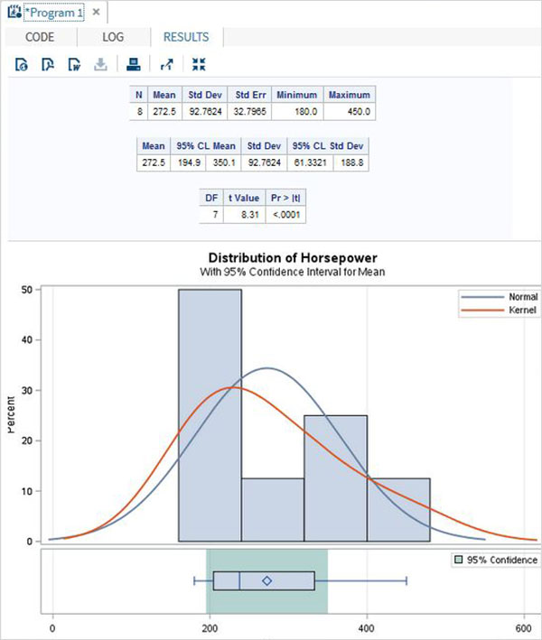
Paired T-test

The paired T Test is carried out to test if two dependent variables are statistically different from each other or not.

Example

As length and weight of a car will be dependent on each other we apply the paired T test as shown below.

proc ttest data = cars1 ;
   paired weight*length;
   run;

When the above code is executed, we get the following result −

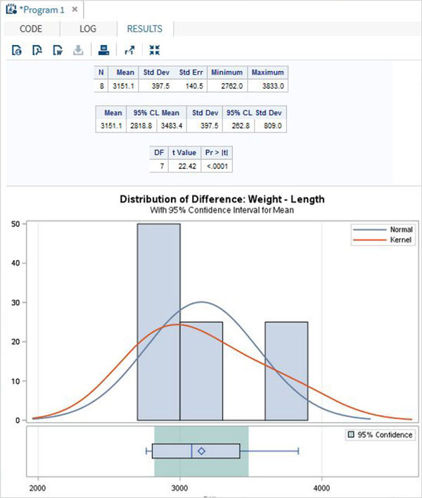
Two sample t-test

This t-test is designed to compare means of same variable between two groups.

Example

In our case we compare the mean of the variable horsepower between the two different makes of the cars("Audi" and "BMW").

proc ttest data = cars1 sides = 2 alpha = 0.05 h0 = 0;
   title "Two sample t-test example";
   class make; 
   var horsepower;
   run;

When the above code is executed, we get the following result −

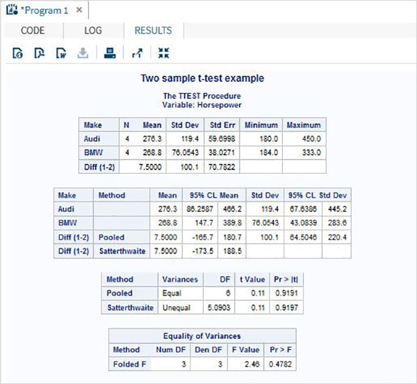
SAS - Correlation Analysis

Correlation analysis deals with relationships among variables. The correlation coefficient is a measure of linear association between two variables.Values of the correlation coefficient are always between -1 and +1. SAS provides the procedure PROC CORR to find the correlation coefficients between a pair of variables in a dataset.

Syntax

The basic syntax for applying PROC CORR in SAS is −

PROC CORR DATA = dataset options;
VAR variable;

Following is the description of the parameters used −

Dataset is the name of the dataset.
Options is the additional option with procedure like plotting a matrix etc.
Variable is the variable name of the dataset used in finding the correlation.

Example

Correlation coefficients between a pair of variables available in a dataset can be obtained by use their names in the VAR statement.In the below example we use the dataset CARS1 and get the result showing the correlation coefficients between horsepower and weight.

PROC SQL;
create table CARS1 as
SELECT invoice, horsepower, length, weight
   FROM 
   SASHELP.CARS
   WHERE make in ('Audi','BMW')
;
RUN;

proc corr data = cars1 ;
VAR horsepower weight ;
BY make;
run;

When the above code is executed, we get the following result −

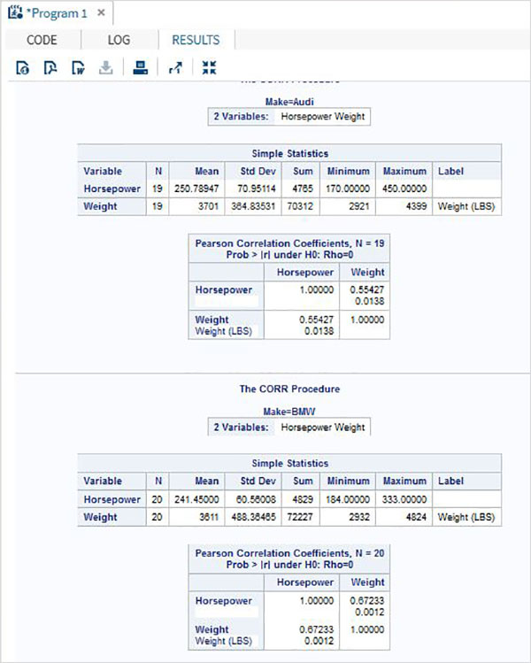
Correlation Between All Variables

Correlation coefficients between all the variables available in a dataset can be obtained by simply applying the procedure with the dataset name.

Example

In the below example we use the dataset CARS1 and get the result showing the correlation coefficients between each pair of the variables.

proc corr data = cars1 ;
run;

When the above code is executed, we get the following result −

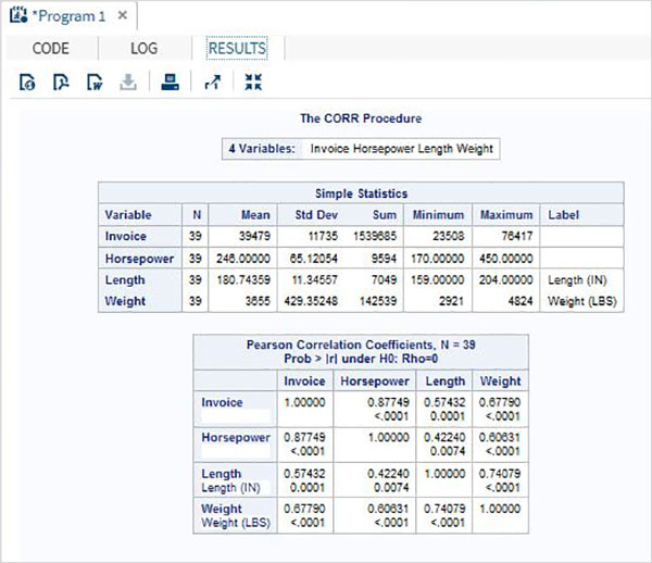
Correlation Matrix

We can obtain a scatterplot matrix between the variables by choosing the option to plot matrix in the PROC statement.

Example

In below example we get the matrix between horsepower and weight.

proc corr data = cars1 plots = matrix ;
VAR horsepower weight ;
run;

When the above code is executed, we get the following result −

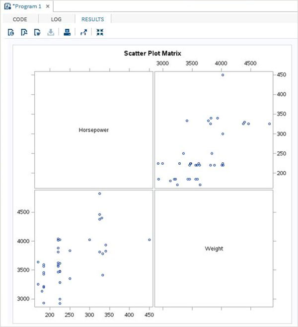
SAS - Linear Regression

Linear Regression is used to identify the relationship between a dependent variable and one or more independent variables. A model of the relationship is proposed, and estimates of the parameter values are used to develop an estimated regression equation.

Various tests are then used to determine if the model is satisfactory. If it is then, the estimated regression equation can be used to predict the value of the dependent variable given values for the independent variables. In SAS the procedure PROC REG is used to find the linear regression model between two variables.

Syntax

The basic syntax for applying PROC REG in SAS is −

PROC REG DATA = dataset;
MODEL variable_1 = variable_2;

Following is the description of the parameters used −

Dataset is the name of the dataset.
variable_1 and variable_2 are the variable names of the dataset used in finding the correlation.

Example

The below example shows the process to find the correlation between the two variables horsepower and weight of a car by using PROC REG. In the result we see the intercept values which can be used to form the regression equation.

PROC SQL;
create table CARS1 as
SELECT invoice, horsepower, length, weight
   FROM 
   SASHELP.CARS
   WHERE make in ('Audi','BMW')
;
RUN;
proc reg data = cars1;
model horsepower = weight ;
run;

When the above code is executed, we get the following result −

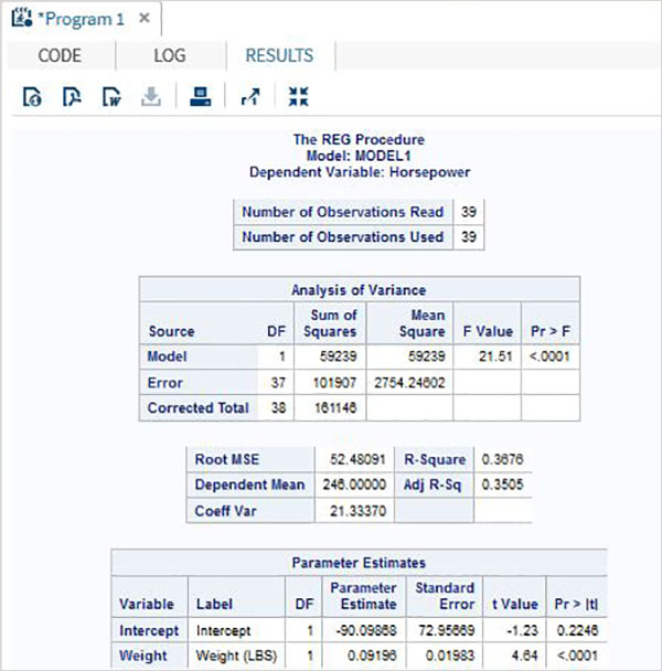
The above code also gives the graphical view of various estimates of the model as shown below. Being an advanced SAS procedure it simply does not stop at giving the intercept values as the output.

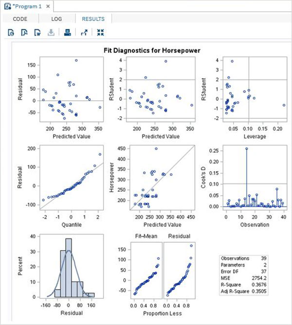
SAS - Bland Altman Analysis

The Bland-Altman analysis is a process to verify the extent of agreement or disagreement between two methods designed to measure same parameters. A high correlation between the methods indicate that good enough sample has been chosen in data analysis. In SAS we create a Bland-Altman plot by calculating the mean, upper limit and lower limit of the variable values. We then use PROC SGPLOT to create the Bland-Altman plot.

Syntax

The basic syntax for applying PROC SGPLOT in SAS is −

PROC SGPLOT DATA = dataset;
SCATTER X = variable Y = Variable;
REFLINE value;

Following is the description of the parameters used −

Dataset is the name of the dataset.
SCATTER statement cerates the scatter plot graph of the value supplied in form of X and Y.
REFLINE creates a horizontal or vertical reference line.

Example

In the below example we take the result of two experiments generated by two methods named new and old. We calculate the differences in the values of the variables and also the mean of the variables of the same observation. We also calculate the standard deviation values to be used in the upper and lower limit of the calculation.

The result shows a Bland-Altman plot as a scatter plot.

data mydata;
input new old;
datalines;
31 45
27 12
11 37
36 25
14 8
27 15
3 11
62 42
38 35
20 9
35 54
62 67
48 25
77 64
45 53
32 42
16 19
15 27
22 9
8 38
24 16
59 25
;

data diffs ;
set mydata ;
/* calculate the difference */
diff = new-old ;
/* calculate the average */
mean = (new+old)/2 ;
run ;
proc print data = diffs;
run;

proc sql noprint ;
select mean(diff)-2*std(diff),  mean(diff)+2*std(diff)
into   :lower,  :upper 
from diffs ;
quit;

proc sgplot data = diffs ;
scatter x = mean y = diff;
refline 0 &upper &lower / LABEL = ("zero bias line" "95% upper limit" "95%
lower limit");
TITLE 'Bland-Altman Plot';
footnote 'Accurate prediction with 10% homogeneous error'; 
run ;
quit ;

When the above code is executed, we get the following result −

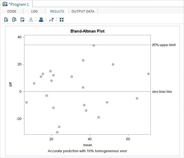
Enhanced Model

In an enhanced model of the above program we get 95 percent confidence level curve fitting.

proc sgplot data = diffs ;
reg x = new y = diff/clm clmtransparency = .5;
needle x = new y = diff/baseline = 0;
refline 0 / LABEL = ('No diff line');
TITLE 'Enhanced Bland-Altman Plot';
footnote 'Accurate prediction with 10% homogeneous error'; 
run ;
quit ;

When the above code is executed, we get the following result −

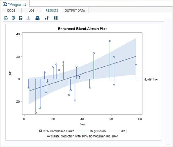
SAS - Chi Square

A chi-square test is used to examine the association between two categorical variables. It can be used to test both extent of dependence and extent of independence between Variables. SAS uses PROC FREQ along with the option chisq to determine the result of Chi-Square test.

Syntax

The basic syntax for applying PROC FREQ for Chi-Square test in SAS is −

PROC FREQ DATA = dataset;
TABLES variables 
/CHISQ TESTP = (percentage values);

Following is the description of the parameters used −

Dataset is the name of the dataset.
Variables are the variable names of the dataset use in chi-square test.
Percentage Values in the TESTP statement represent the percentage of levels of the variable.

Example

In the below example we consider a chi-square test on the variable named type in the dataset SASHELP.CARS. This variable has six levels and we assign percentage to each level as per the design of the test.

proc freq data = sashelp.cars;
tables type 
/chisq 
testp = (0.20 0.12 0.18 0.10 0.25 0.15);
run;

When the above code is executed, we get the following result −

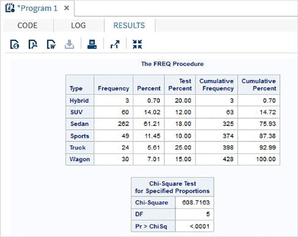
We also get the bar chart showing the deviation of the variable type as shown in the following screenshot.

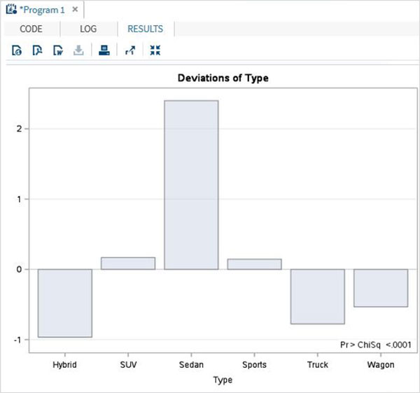
Two Way chi-square

Two way Chi-Square test is used when we apply the tests to two variables of the dataset.

Example

In the below example we apply chi-square test on two variables named type and origin. The result shows the tabular form of all combinations of these two variables.

proc freq data = sashelp.cars;
tables type*origin 
/chisq 
;
run;

When the above code is executed, we get the following result −

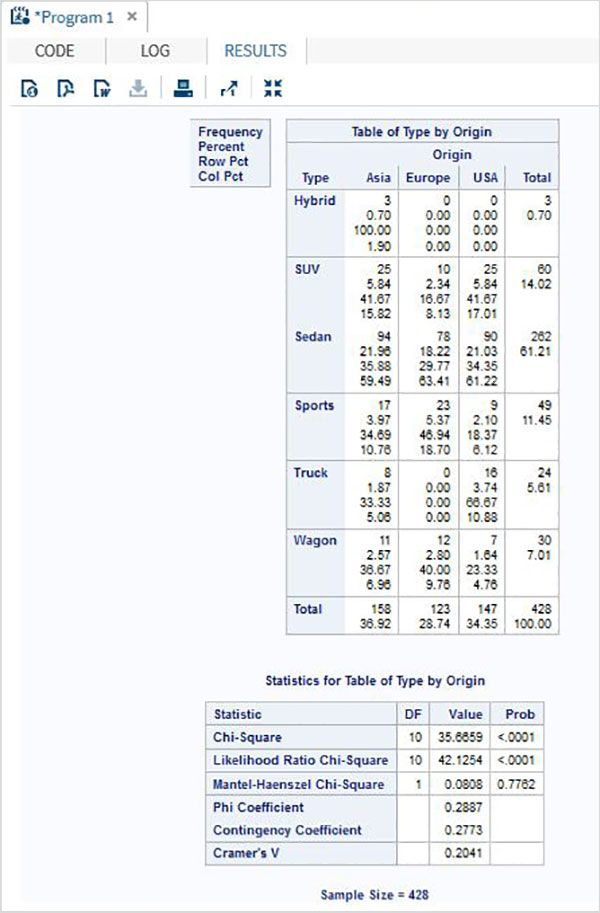
SAS - Fishers Exact Tests

Fisher's exact test is a statistical test used to determine if there are nonrandom associations between two categorical variables.In SAS this is carried out using PROC FREQ. We use the Tables option to use the two variables subjected to Fisher Exact test.

Syntax

The basic syntax for applying Fisher Exact test in SAS is −

PROC FREQ DATA = dataset ;
TABLES Variable_1*Variable_2 / fisher;

Following is the description of the parameters used −

dataset is the name of the dataset.
Variable_1*Variable_2 are the variables form the dataset .

Applying Fisher Exact Test

To apply Fisher's Exact Test, we choose two categorical variables named Test1 and Test2 and their result.We use PROC FREQ to apply the test shown below.

Example

data temp;
input  Test1 Test2 Result @@;
datalines;
1 1 3 1 2 1 2 1 1 2 2 3
;
proc freq; 
tables Test1*Test2 / fisher;
run;

When the above code is executed, we get the following result −

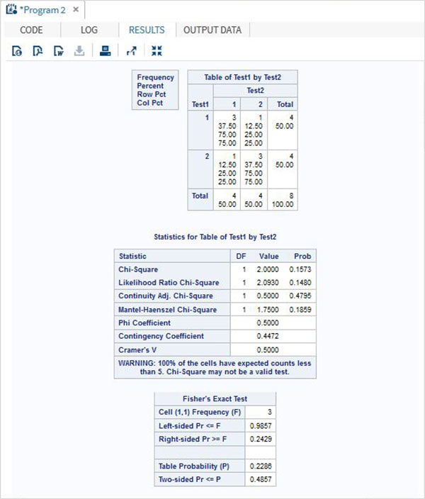
SAS - Repeated Measure Analysis

Repeated measure analysis is used when all members of a random sample are measured under a number of different conditions. As the sample is exposed to each condition in turn, the measurement of the dependent variable is repeated. Using a standard ANOVA in this case is not appropriate because it fails to model the correlation between the repeated measures.

One should be clear about the difference between a repeated measures design and a simple multivariate design. For both, sample members are measured on several occasions, or trials, but in the repeated measures design, each trial represents the measurement of the same characteristic under a different condition.

In SAS PROC GLM is used to carry out repeated measure analysis.

Syntax

The basic syntax for PROC GLM in SAS is −

PROC GLM DATA = dataset;
   CLASS variable;
   MODEL variables = group / NOUNI;
   REPEATED TRIAL n;

Following is the description of the parameters used −

dataset is the name of the dataset.
CLASS gives the variables the variable used as classification variable.
MODEL defines the model to be fit using certain variables form the dataset.
REPEATED defines the number of repeated measures of each group to test the hypothesis.

Example

Consider the example below in which we have two groups of people subjected to test of effect of a drug. The reaction time of each person is recorded for each of the four drug types tested. Here 5 trials are done for each group of people to see the strength of correlation between the effect of the four drug types.

DATA temp;
   INPUT person group $ r1 r2 r3 r4;
CARDS;
1 A  2  1  6  5
2 A  5  4 11  9
3 A  6 14 12 10
4 A  2  4  5  8
5 A  0  5 10  9
6 B  9 11 16 13
7 B  12 4 13 14
8 B  15 9 13  8
9 B  6  8 12  5
10 B 5  7 11  9
;
RUN;

PROC PRINT DATA = temp ;
RUN;

   PROC GLM DATA = temp;
   CLASS group;
   MODEL r1-r4 = group / NOUNI ;
   REPEATED trial 5;
RUN;

When the above code is executed, we get the following result −

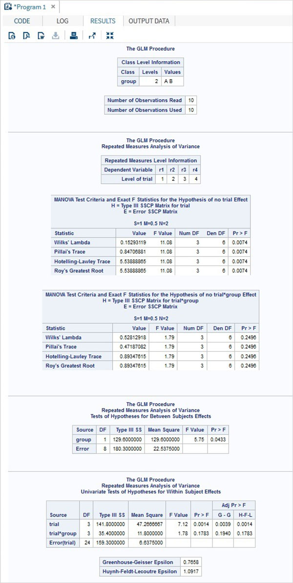
SAS - One Way Anova

ANOVA stands for Analysis of Variance. In SAS it is done using PROC ANOVA. It performs analysis of data from a wide variety of experimental designs. In this process, a continuous response variable, known as a dependent variable, is measured under experimental conditions identified by classification variables, known as independent variables. The variation in the response is assumed to be due to effects in the classification, with random error accounting for the remaining variation.

Syntax

The basic syntax for applying PROC ANOVA in SAS is −

PROC ANOVA dataset ;
CLASS Variable;
MODEL Variable1 = variable2 ;
MEANS ;

Following is the description of the parameters used −

dataset is the name of the dataset.
CLASS gives the variables the variable used as classification variable.
MODEL defines the model to be fit using certain variables from the dataset.
Variable_1 and Variable_2 are the variable names of the dataset used in analysis.
MEANS defines the type of computation and comparison of means.

Applying ANOVA

Let us now understand the concept of applying ANOVA in SAS.

Example

Lets consider the dataset SASHELP.CARS. Here we study the dependence between the variables car type and their horsepower. As the car type is a variable with categorical values, we take it as class variable and use both these variables in the MODEL.

PROC ANOVA DATA = SASHELPS.CARS;
CLASS type;
MODEL horsepower = type;
RUN;

When the above code is executed, we get the following result −

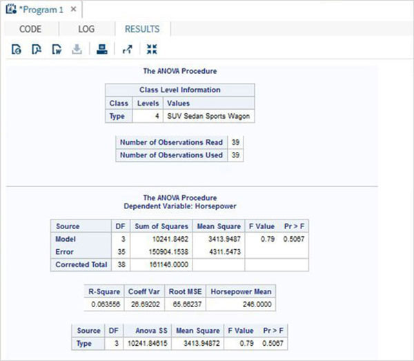
Applying ANOVA with MEANS

Let us now understand the concept of applying ANOVA with MEANS in SAS.

Example

We can also extend the model by applying the MEANS statement in which we use Turkey's Studentized method to compare the mean values of various car types.The category of car types are listed with the mean value of horsepower in each category along with some additional values like error mean square etc.

PROC ANOVA DATA = SASHELPS.CARS;
CLASS type;
MODEL horsepower = type;
MEANS type / tukey lines;
RUN;

When the above code is executed, we get the following result −

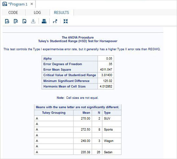
SAS - Hypothesis Testing

Hypothesis testing is the use of statistics to determine the probability that a given hypothesis is true. The usual process of hypothesis testing consists of four steps as shown below.

Step-1

Formulate the null hypothesis H0 (commonly, that the observations are the result of pure chance) and the alternative hypothesis H1 (commonly, that the observations show a real effect combined with a component of chance variation).

Step-2

Identify a test statistic that can be used to assess the truth of the null hypothesis.

Step-3

Compute the P-value, which is the probability that a test statistic at least as significant as the one observed would be obtained assuming that the null hypothesis were true. The smaller the P-value, the stronger the evidence against the null hypothesis.

Step-4

Compare the p-value to an acceptable significance value alpha (sometimes called an alpha value). If p <=alpha, that the observed effect is statistically significant, the null hypothesis is ruled out, and the alternative hypothesis is valid.

SAS programming language has features to carry out various types of hypothesis testing as shown below.

Test	Description	SAS PROC
T-Test	A t-tests is used to test whether the mean of one variable is significantly different than a hypothesized value.We also determine whether means for two independent groups are significantly different and whether means for dependent or paired groups are significantly different.	PROC TTEST
ANOVA	It is also used to compare means when there is one independent categorical variable. We want to use one-way ANOVA when testing to see if the means of the interval dependent variable are different according to the independent categorical variable.	PROC ANOVA
Chi-Square	We use chi square goodness of fit to assess if frequencies of a categorical variable were likely to happen due to chance. Use of a chi square test is necessary whether proportions of a categorical variable are a hypothesized value.	PROC FREQ
Linear Regression	Simple linear regression is used when one wants to test how well a variable predicts another variable. Multiple linearregression allows one to test how well multiple variables predict a variable of interest. When using multiple linear regression, we additionally assume the predictor variables are independent.	PROC REG

SAS - Quick Guide

SAS - Overview

Why we use SAS

Types of SAS Software

Libraries in SAS

SAS - Environment

Download SAS University Edition

Setup virtualization software

Quick start virtualization software

Download the Zip file

Unzip the zip file

Loading the virtual machine

Power on the virtual machine

Starting SAS studio

The SAS Environment

SAS - User Interface

SAS Main Window

Code Autocomplete

Program Execution

Program Log

Program Result

Program Tabs

Server Files and Folders

Tasks

Snippets

Program Libraries

File Shortcuts

SAS - Program Structure

SAS Program Structure

DATA Step

Syntax

Example

PROC Step

Syntax

Example

The OUTPUT Step

Syntax

Example

The complete SAS Program

Program Output

SAS - Basic Syntax

SAS Statements

SAS Variable Names

Example

SAS Data Set

Example

SAS File Extensions

Comments in SAS

*message; type comment

/*message*/ type comment

SAS - Data Sets

SAS Built-In Data Sets

Importing External Data Sets

View the imported data

SAS - Variables

SAS Variable Types

Numeric Variables

Syntax

Example

Character Variables

Syntax

Example

Date Variables

Syntax

Example

Use of Variables in SAS Program

Example

Using the Variables

SAS - Strings

Declaring String Variables

String Functions

SUBSTRN

Syntax

Example

TRIMN

Syntax

SAS - Arrays

Syntax

Examples of Array Declaration

Accessing Array Values

/message/ type comment