Calculus -Differentiation

Description:

Differential Calculus

• Calculus is a branch of Mathematics and a vast domain in itself. You will study calculus in detail in 12^th standard Mathematics.

• Calculus has extensive use in Physics in all of its domains.

• Differential Calculus is majorly used as a rate measurement tool.

Case Study – Car moving on a straight road

Constant Speed motion

• Let’s say a car is moving on a straight road at constant speed.

• The Distance vs Time plot for the same would look like follows −

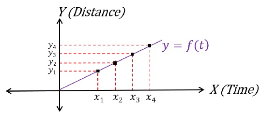
• Car is covering equal distances in equal time because it is going at a constant speed.

• Therefore, one can say,

  (y₁ - 0)/(x₁ - 0) = (y₂ - y₁)/(x₂ - x₁) = (y₃ - y₂)/(x₃ - x₂) = (y₄ - y₃)/(x₄ - x₃) = Constant

• Rate of change of distance with respect to time is always same.

Increasing/Non-constant Speed motion

• The same car starts to increase its speed of motion.

• Now, let’s say, the Distance vs Time plot would look like follows −

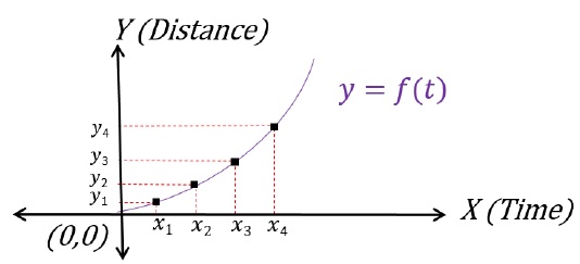
• Car is DOES NOT cover equal distances in equal time because its speed is increasing. In fact, the car covers the larger distances every unit time.

• Therefore, one can say,

  (y₁ - 0)/(x₁ - 0) ≠ (y₂ - y₁)/(x₂ - x₁) ≠ (y₃ - y₂)/(x₃ - x₂) ≠ (y₄ - y₃)/(x₄ - x₃)

• Rate of change of distance with respect to time is never same.

Mathematical Analysis of Rate of Change

• Consider any two arbitrary points (x₁,y₁) and (x₂,y₂) on the plot.

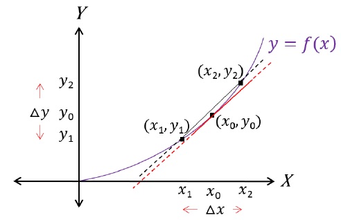
• Between points (x₁,y₁) and (x₂,y₂), the rate of change can be defined as −

  Average Rate of Change = (y₂ - y₁)/(x₂ - x₁) = Δy/Δx

• The result of this average rate of change can be taken as the average speed of the car.

• However, the plot of the motion is not really a straight line but, a curve.

• Therefore, we are also interested in the value of speed (rate of change of distance w.r.t. time) at every instant (of time) and, not just the average.

• We define instantaneous speed of the car at x = x₀ as follows −

• To physically visualize this, imagine that we start bringing our reference points (x₁,y₁) and (x₂,y₂) closer to each other on the curve towards (x₀,y₀).

• When they are very, very close to (x₀,y₀), the value of both Δx and Δy are very, very close to zero.

• The three points are so close that they are almost on a straight line now and there is no curvature left.

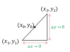
• At this point, the rate of change can be defined as −

  Rate of Change = lim(x₂ - x₁)→0(y₂ - y₁)/(x₂ - x₁) = limΔx→0Δy/Δx = dy/dx

• ‘dy’ and ‘dx’ represent infinitesimally small change in ‘y’ and ‘x’ respectively.

• This rate of change obtained can also be called the instantaneous rate of change or, instantaneous speed of the car in the case study.

• Therefore,

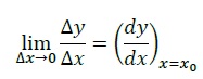
  Instantaneous rate of Change = limΔx→0Δy/Δx = (dy/dx)_{x = x0}

Relating these results to the moving car case study,

Average Speed of the car between time x₁ and x₂ = (y₂ - y₁)/(x₂ - x₁) = Δy/Δx

Instantaneous speed of the car at x₀ = limΔx→0Δy/Δx = (dy/dx)_{x = x0}

(dy/dx)as the slope of the tangent

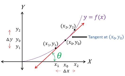
• dy/dx can also be understood as the slope of the tangent to the curve at x = x₀.

• This is so because dy/dx is nothing but extremely small value of (y₂ - y₁) divided by extremely small value of (x₂ - x₁).

• Slope of the tangent is defined as: slope = tan θ, where ‘θ’ is the angle tangent makes with the positive x − axis.

• You will learn more about slope in Straight Lines chapter of Mathematics.

(dy/dx) of some common functions

• If y = c where c ∈ constant, then dy/dx = dc/dx = 0

• If y = xⁿ, then dy/dx = d/dx (xⁿ) = n x^(n-1)

• If y = e^x, where "e" is euler′s constant, then dy/dx = d/dx (e^x) = e^x

• If y = a^x, where a ∈ constant, then dy/dx = d/dx (a^x) = a^x ln(a)

• If y = log_ex = ln x, where "e" is euler′s constant, then dy/dx = d/dx (ln x) = 1/x

• If y = log_a x, where a ∈ constant, then dy/dx = d/dx (log_ax) = 1/x ln a

• If y = sinx, then dy/dx = d/dx (sin x) = cos x

• If y = cos x, then dy/dx = d/dx (cos x) = - sin x

• If y = tan x, then dy/dx = d/dx (tanx) = sec²x

• If y = cosec x, then dy/dx = d/dx (cosec x) = - cosec x cot x

• If y = sec x, then dy/dx = d/dx (sec x) = sec x tan x

• If y = cot x, then dy/dx = d/dx (cot x) = - cosec²x

Addition, Subtraction, Multiplication, Division Rules

• d(u ± v)/dx = du/dx ± dv/dx

• d(u x v)/dx = u dv/dx + v du/dx

• d(u/v)/dx = v du/dx - u dv/dx/v²

How to use the formulae - Example

Differentiate: y = sin x + x³ ln x + e^x tan x

• dy/dx = d(sin x)/dx + d(x³ ln x)/dx + d(e^x tan x)/dx

• dy/dx = cos x + (ln xd(x³)/dx + x³ d(ln x)/dx) + (tan xd(e^x)/dx + e^x d(tan x)/dx)

• dy/dx cos x + (ln x (3x²) + (x³)1/x) + (tan x(e^x) + e^x(sec²x))

• dy/dx = cos x + (3x² ln x + x²) + (e^xtan x + e^x sec²x)

Chain Rule

Let’s say, y = f(t) and x = g(t).

• Both the variables are functions of ‘t’.

• If we have to calculate dy/dx, then following method is used −

  dy/dx = dy/dt x dt/dx

• This can also be written as −

  dy/dx = dy/dt x 1/dx/dt

• Values of dy/dt and dx/dt can be calculated using the formulae mentioned previously.

Chain Rule - Example

Lets say, y = sin t and x = cos t.

• Then dy/dx −

  dy/dx = d(sin t)/dt x dt/d(cos t)

This can also be written as −

dy/dx = d(sin t)/dt x (1/d(cos t)/dt)

dy/dx = cos t x (1/- sin t)

dy/dx = - (cos t/sin t) = - cot(t) = - cot(cos^-1x) = - cot(sin^-1y)