Calculus - Integration

Description:
Integral Calculus
Calculus is a branch of Mathematics and a vast domain in itself. You will study calculus in detail in 12th standard Mathematics.
Calculus has extensive use in Physics in all of its domains.
Integral calculus is majorly used −
As a reverse process of differentiation
For calculating area under the curve/graph of any function.
Indefinite Integration
Indefinite Integration can be understood as the reverse process of differentiation.
For any function y = F(x);
If, dydx = f(x),
Then ∫ f(x) . dx = F(x) + c [c ∈ constant of integration]
The symbol ‘∫’ represents the operation of integration.
The ′c′ value allows us to obtain a family of curves which have the same derivative. Let’s understand the statement −
Derivative of any constant number is 0(Zero).
Therefore, ddx(F(x) + c) = ddx (F(x)) + ddx (c) = f(x) + 0 = f(x)
Therefore, logically, ∫ f(x) . dx = F(x) + c and NOT F(x).
Family of curves look like following: (c = 1,2,3,4,etc.,)
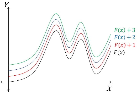
Derivative of each curve shown here is f(x).
Example
Let’s say y = tan x;
Then, dydx = sec2x;
Therefore
∫ sec2x . dx = (tan x) + c [c ∈ constant of integration]
Indefinite Integration – Formulae
∫ a . dx = ax + c, where a, c ∈ constant
∫ xn . dx = xn+1n+1 + c, where n, c ∈ constant
∫ ex . dx = ex + c, where e is euler′s constant, c ∈ constant
∫ ax . dx = axln a + c, where a, c ∈ constant
∫ 1x . dx = ln x + c = logex + c, where e is euler′s constant
∫ 1x ln a . dx = logax + c, where a, c ∈ constant
∫ sin x . dx = - cos x + c, where c ∈ constant
∫ cos x. dx = - sin x + c, where c ∈ constant
∫ sec2x . dx = tan x + c, where c ∈ constant
∫ - cosec x cot x . dx = cosec x + c, where c ∈ constant
∫ sec x tan x . dx = sec x + c, where c ∈ constant
∫ - cosec2x . dx = cot x + c, where c ∈ constant
Addition and Subtraction Rules
Let’s say, u = f(x) and v = g(x).
∫ (u ± v) . dx = ∫ u . dx ± ∫ v . dx
There is no direct multiplication or division rule, unlike differentiation.
Example
Integrate: y = sin x + x3 + ex
∫ y . dx = ∫ (sin x + x3 + ex) . dx
This implies, ∫ y . dx = ∫ sin x dx + ∫ x3 . dx + ∫ ex . dx
This implies, ∫ y . dx = - cos x + x44 + ex + c
Definite Integration
Definite Integration could be used to calculate the area under any curve. It could be understood as a limit of the sum. Consider the following curve y = f(x). Our goal is to find the area under the curve between x = 0 and x = x0.
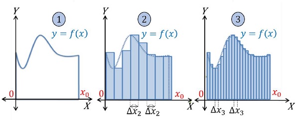
No.1 plot shows the function y = f(x).
No.2 plot shows an attempt to approximate the area under the curve by using rectangular bars.
Let’s say the width of each bar is Δx2.
Total n2 such bars are needed to cover the area.
Approximate area under the curve: n=n2∑n=0 yΔx2
No.3 plot is more accurate approximation of area with respect to No.2.
Let’s say the width of each bar is Δx3.
Total n3 such bars are needed to cover the area.
Approximate area under the curve: n=n3∑n=0 yΔx3
If one decreases the width of each bar (thereby increasing the number of bars required), they will reach to a point when the area defined by the bars is almost accurate.
In that limiting situation (when the area obtained is accurate),
The width of each bar will be very small (almost zero), hence Δx → 0
The number of bars required will be very large (almost infinity), hence n → ∞.
Therefore,
limn→∞, Δx→0n=n∑n=0 yΔx = x0∫0 y . dx (Δx changes into dx)
Definite integrals have upper and lower limits present on them. As one can see in the above equation, the lower limit is 0(zero) and the upper limit is x0.
Definite Integration – General Form
For a function, y = f(x), definite integral is defined as −
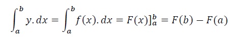
Here,
′a′ is the lower limit and ′b′ is the upper limit of integral.
F(x) is the function obtained as the result of integration.
The result also indicates the area under of the curve of y = f(x), between x = a and x = b.
All the formulae of indefinite integration is applicable to definite integration as well.
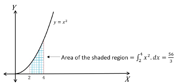
Definite Integration – Example
For a function, y = x2, find 4∫2 y . dx
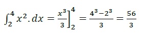
This also represents area under the curve of y = x2 between x = 2 and x = 4.