Electric Field Due to Charged Long Conductor

Description:

Let there be an infinitely large conductor in which charges are uniformly distributed  and we are supposed to find electric field at a certain distance ‘r’ at point ‘P’ using Gauss Theorem.

We know that if the charge distribution is over a line then we use linear charge density (λ) to find the electric field.

Step 1

We take a cylindrical Gaussian surface of radius ‘r’ and length ‘l’, With conductor as its axis and P lies on the surface. as shown in figure. E→ is radial (perpendicular to charged surface) is symmetrical at every point of curved surface .  Area vector A→ makes an angle 0. With  electric field E→. At every point on the curved surface.

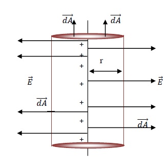
Flat surfaces is also a part of Gaussian surface. But the area vector(A→) always makes 90^o. With electric field vector (E→). so this arises the question on the symmetry of Gaussian surface.

So, according to the derived rule, whenever we cannot imagine one surface which is completely symmetric then we divide the Gaussian surface into two surfaces so that each surface has separate symmetry.

So in case of a line charged conductor with cylindrical Gaussian surface , electric field at every point on the curved surface is 0^o, whereas at every point on flat surface is 90^o. Hence both the surface makes a perfect symmetry.

Step 2

If there are more than one symmetry the calculation of electric flux is done separately for each surface and all are then added up to get total electric flux.

Φ = ∮ E→.dA→ = ∮ EdScos θ

⇒ Φ = ∮ EdScos 0 + ∮ EdScos 90 + ∮ EdScos 90

⇒ Φ = E ∮ dS

So ∮ dS = 2 πrl

So, Φ = E 2πrl

Step 3

Charge on 1m = λ

So charge on lm = l λ

Charge within the surface = 1 λ

Step 4

Apply Gauss Theorem −

∮ E→.dA→ = q/ ε₀

Putting values in the equation we get −

E 2πrl = 1 λ/ ε₀

So, E = 1/2πε₀ λ/r